# Uncomment this cell if running in Google Colab
!pip install clinicadl==1.6.1

Training for reconstruction#

The objective of the reconstruction is to learn to reconstruct images given as input. To do so, we can use a type of artificial neural network called autoencoder.

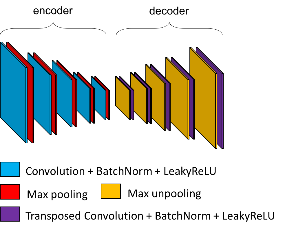
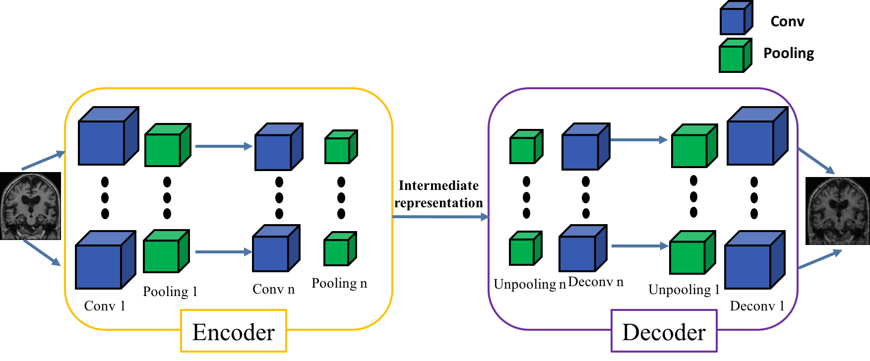
An autoencoder learns to reconstruct data given as input. It is composed of two parts:

The encoder which reduces the dimensionality of the input to a smaller feature map: the code.
The decoder which reconstructs the input based on the code.

The mean squared error is used to evaluate the difference between the input and its reconstruction.

There are many paradigms associated to autoencoders, but here we will only focus on a specific case that allows us to get the weights that can be transferred to a CNN. In ClinicaDL, the autoencoders are designed based on a CNN:

the encoder corresponds to the convolutional layers of the CNN,
the decoder is composed of the transposed version of the operations used in the encoder.

After training the autoencoder, the weights in its encoder can be copied in the convolutional layers of a CNN to initialize it. This can improve its performance as the autoencoder has already learnt patterns characterizing the data distribution.

*Autoencoder derived from the previous CNN architecture*

3D patch-level & ROI-based models#

The 3D patch-level models compensate the absence of 3D information in the 2D slice-level approach and keep some of its advantages (low memory usage and larger sample size).

ROI-based models are similar to 3D-patch but take advantage of prior knowledge on Alzheimer’s disease. Indeed most of the patches are not informative as they contain parts of the brain that are not affected by the disease. Methods based on regions of interest (ROI) overcome this issue by focusing on regions which are known to be informative: here the hippocampi. In this way, the complexity of the framework can be decreased as fewer inputs are used to train the networks.

3D patch-level tensor extraction with the `prepare-data` pipeline#

Before starting, we need to obtain files suited for the training phase. This pipeline prepares images generated by Clinica to be used with the PyTorch deep learning library (Paszke et al., 2019). Four types of tensors are proposed: 3D images, 3D patches, 3D ROI or 2D slices.

This pipeline selects the preprocessed images, extract the “tensors”, and write them as output files for the entire images, for each slice, for each roi or for each patch.

Here, as you will use slice-level, you simply need to type the following command line:

clinicadl prepare-data patch <caps_directory> <modality>

where:

caps_directory is the folder containing the results of the t1-linear pipeline and the output of the present command, both in a CAPS hierarchy.
modality is the name of the preprocessing performed on the original images. It can be t1-linear or pet-linear. You can choose custom if you want to get a tensor from a custom filename.

When using patch or slice extraction, default values were set according to Wen et al., 2020

Output files are stored into a new folder (inside the CAPS) and follows a structure like this:

deeplearning_prepare_data
├── image_based
│   └── t1_linear
│       └── sub-<participant_label>_ses-<session_label>_T1w_space-MNI152NLin2009cSym_desc-Crop_res-1x1x1_T1w.pt
└── patch_based
    └── t1_linear
        ├── sub-<participant_label>_ses-<session_label>_T1w_space-MNI152NLin2009cSym_desc-Crop_res-1x1x1_axis-axi_channel-rgb_patch-0_T1w.pt
        ├── sub-<participant_label>_ses-<session_label>_T1w_space-MNI152NLin2009cSym_desc-Crop_res-1x1x1_axis-axi_channel-rgb_patch-1_T1w.pt
        ├── ...
        └── sub-<participant_label>_ses-<session_label>_T1w_space-MNI152NLin2009cSym_desc-Crop_res-1x1x1_axis-axi_channel-rgb_patch-N_T1w.pt

In short, there is a folder for each feature (image, slice, roi or patch) and inside the numbered tensor files with the corresponding feature. Files are saved with the .pt extension and contains tensors in PyTorch format. A JSON file is also stored in the CAPS hierarchy under the tensor_extraction folder:

CAPS_DIRECTORY
└── tensor_extraction
        └── <extract_json>

These files are compulsory to run the train command. They provide all the details of the processing performed by the prepare-data command that will be necessary when reading the tensors.

Warning

The default behavior of the pipeline is to only extract images even if another extraction method is specified. However, all the options will be saved in the preprocessing JSON file and then the extraction is done when data s loaded during the training. If you want to save the extracted method tensors in the CAPS, you have to add the --save-features flag.

ClinicaDL is able to extract patches on-the-fly (from one single file) when running training or inference tasks. The downside of this approach is that, depending on the size of your dataset, you have to make sure that you have enough memory resources in your GPU card to host the full images/tensors for all your data.

If the memory size of the GPU card you use is too small, we suggest you to extract the patches and/or the slices using the proper tensor_format option of the command described above.

(If you failed to obtain the preprocessing using the t1-linear pipeline, please uncomment the next cell)

!curl -k https://aramislab.paris.inria.fr/clinicadl/files/handbook_2023/CAPS_example.tar.gz -o oasisCaps.tar.gz
!tar xf oasisCaps.tar.gz

To perform the feature extraction for our dataset, run the following cell:

!clinicadl prepare-data patch data_oasis/CAPS_example pet-linear --subjects_sessions_tsv data_adni/after_qc.tsv --extract_json pet_reconstruction --acq_label 18FFDG --suvr_reference_region cerebellumPons2

At the end of this command, a new directory named deeplearning_prepare_data is created inside each subject/session of the CAPS structure. We can easily verify:

!tree -L 3 ./data_oasis/CAPS_example/subjects/sub-OASIS10*/ses-M00/deeplearning_prepare_data/

# We can also do the same things with region of interest. 
# ROI are 3D patches defined by masks that need to be at the root in
# `CAPS_DIRECTORY`. 
# In the data_adni/masks folder you can find masks of the right and left
# hippocampus that can be used to define two region of interest.
#
# Uncomment the next cell if you want to extract roi tensors:

!cp -r data/masks data_adni/CAPS_example/masks
!clinicadl prepare-data roi data_adni/CAPS_example pet-linear --roi_list rightHippocampusBox --roi_list leftHippocampusBox

These two paradigms can be divided into two different frameworks:

single-network: one network is trained on all patch locations / all regions.
multi-network: one network is trained per patch location / per region.

For multi-network the sample size is smaller (equivalent to image level framework), however the network may be more accurate as they are specialized for one patch location / for one region.

As for the 2D slice-level model, the gradient updates are done based on the loss computed at the patch level. Final performance metrics are computed at the subject level by combining the outputs of the patches or the two hippocampi of the same subject.

The default network used for reconstruction in ClinicaDL is an autoencoder derived from the convolutional part of CNN with 5 convolutionnal layers followed by 3 fully connected. The compatible criterion loss are :

the mean squared error between the input and the network output (link),
the Kullback-Leibler divergence loss (link),
the mean absolute error loss (link),
a combination of a Sigmoid layer and the BCELoss (link),
the Huber loss (link),
the smooth L1 loss (link) but the default one is the mean square error.

The evaluation metrics are the mean squared error (MSE) and mean absolute error (MAE).

Before starting#

Warning

If you do not have access to a GPU, training the CNN may require too much time. However, you can execute this notebook on Colab to run it on a GPU.

If you already know the models implemented in clinicadl, you can directly jump to the train custom to implement your own custom experiment!

from pyrsistent import v
import torch

# Check if a GPU is available
print('GPU is available', torch.cuda.is_available())

Data used for training#

Because they are time-costly, the preprocessing steps presented in the beginning of this tutorial were only executed on a subset of OASIS-1, but obviously two participants are insufficient to train a network! To obtain more meaningful results, you should retrieve the whole OASIS-1 dataset and run the training based on the labels and splits performed in the previous section. Of course, you can use another dataset, but then you will have to perform again “./label_extraction.ipynb” the extraction of labels and data splits on this dataset.

`clinicadl train RECONSTRUCTION`#

This functionality mainly relies on the PyTorch deep learning library [Paszke et al., 2019].

Different tasks can be learnt by a network: classification, reconstruction and regression, in this notebook, we focus on the reconstruction task.

Prerequisites#

You need to execute the clinicadl tsvtool get-labels and clinicadl tsvtools {split|kfold}commands prior to running this task to have the correct TSV file organization. Moreover, there should be a CAPS, obtained running the preprocessing pipeline wanted.

Running the task#

The training task can be run with the following command line:

clinicadl train reconstruction [OPTIONS] CAPS_DIRECTORY PREPROCESSING_JSON \
                TSV_DIRECTORY OUTPUT_MAPS_DIRECTORY

where mandatory arguments are:

CAPS_DIRECTORY (Path) is the input folder containing the neuroimaging data in a CAPS hierarchy. In case of multi-cohort training, must be a path to a TSV file.
PREPROCESSING_JSON (str) is the name of the preprocessing json file stored in the CAPS_DIRECTORY that corresponds to the clinicadl extract output. This will be used to load the correct tensor inputs with the wanted preprocessing.
TSV_DIRECTORY (Path) is the input folder of a TSV file tree generated by clinicadl tsvtool {split|kfold}. In case of[multi-cohort training, must be a path to a TSV file.
OUTPUT_MAPS_DIRECTORY (Path) is the folder where the results are stored.

The training can be configured through a Toml configuration file or by using the command line options. If you have a Toml configuration file you can use the following option to load it:

--config_file (Path) is the path to a Toml configuration file. This file contains the value for the options that you want to specify (to avoid too long command line).

If an option is specified twice (in the configuration file and, as an option, in the command line) then the values specified in the command line will override the values of the configuration file.

A few options depend on the regression task:

--selection_metrics (str) are metrics used to select networks according to the best validation performance. Default: loss.
--loss (str) is the name of the loss used to optimize the reconstruction task. Must correspond to a Pytorch class. Default: MSELoss.

(If you failed to obtain the tensor extraction using the prepare-data pipeline, please uncomment the next cell)

!curl -k https://aramislab.paris.inria.fr/clinicadl/files/handbook_2023/data_adni/CAPS_extracted.tar.gz -o oasisCaps_extracted.tar.gz
!tar xf oasisCaps_extracted.tar.gz

Please note that the purpose of this notebook is not to fully train a network because we don’t have enough data. The objective is to understand how ClinicaDL works and make inferences using pretrained models in the next section.

# 3D-patch autoencoder pretraining
!clinicadl train reconstruction -h
!clinicadl train reconstruction data_adni/CAPS_example pet_reconstruction data_adni/split/4_fold/ data_adni/maps_reconstruction_3D_patch --n_splits 4 

Transfer learning:

It is possible for these categories to train an autoencoder derived from the CNN architecture. The encoder will share the same architecture as the CNN until the fully-connected layers (see the bakground section for more details on autoencoders construction).

Then the weights of the encoder will be transferred to the convolutions of the CNN to initialize it before its training. This procedure is called autoencoder pretraining.

It is also possible to transfer weights between two CNNs with the same architecture.

For 3D-patch multi-CNNs specifically, it is possible to initialize each CNN of a multi-CNN:

with the weights of a single-CNN,
with the weights of the corresponding CNN of a multi-CNN.

Transferring weights between CNNs can be useful when performing two classification tasks that are similar. This is what has been done in (Wen et al., 2020): the sMCI vs pMCI classification network was initialized with the weights of the AD vs CN classification network.

Warning

Transferring weights between tasks that are not similar enough can hurt the performance!

# With autoencoder pretraining
!clinicadl train classification data_adni/CAPS_example pet_reconstruction data_adni/split/4_fold data_adni/maps_classification_3D_patch_transfer --architecture Conv4_FC3 --transfer_path data_adni/maps_reconstrcution_patch --n_splits 4 --epochs 3

# 3D-patch multi-CNN training
!clinicadl train classification -h 

# With autoencoder pretraining
!clinicadl train classification data_adni/CAPS_example pet_reconstruction data_adni/split/4_fold data_adni/maps_classification_transfer_AE_patch_multi --architecture Conv4_FC3 --transfer_path data_adni/maps_reconstrcution_patch --n_splits 4 --epochs 3 --multi-network

The clinicadl train command outputs a MAPS structure in which there are only two data groups: train and validation. A MAPS folder contains all the elements obtained during the training and other post-processing procedures applied to a particular deep learning framework. The hierarchy is organized according to the fold, selection metric and data group used.

An example of a MAPS structure is given below

<maps_directory>
├── environment.txt
├── split-0
│       ├── best-loss
│       │       ├── model.pth.tar
│       │       ├── train
│       │       │       ├── description.log
│       │       │       ├── train_image_level_metrics.tsv
│       │       │       └── train_image_level_prediction.tsv
│       │       └── validation
│       │               ├── description.log
│       │               ├── validation_image_level_metrics.tsv
│       │               └── validation_image_level_prediction.tsv
│       └── training_logs
│               ├── tensorboard
│               │       ├── train
│               │       └── validation
│               └── training.tsv
├── groups
│       ├── train
│       │       ├── split-0
│       │       │       ├── data.tsv
│       │       │       └── maps.json
│       │       └── split-1
│       │               ├── data.tsv
│       │               └── maps.json
│       ├── train+validation.tsv
│       └── validation
│               ├── split-0
│               │       ├── data.tsv
│               │       └── maps.json
│               └── split-1
│                       ├── data.tsv
│                       └── maps.json
└── maps.json

You can find more information about MAPS structure on our documentation

Inference#

(If you failed to train the model please uncomment the next cell)

!curl -k https://aramislab.paris.inria.fr/clinicadl/files/handbook_2023/data_adni/CAPS_example.tar.gz -o adniCaps.tar.gz
!tar xf adniCaps.tar.gz

The predict functionality performs individual prediction and metrics computation on a set of data using models trained with clinicadl train or clinicadl random-search tasks. It can also use any pretrained models if they are structured like a MAPS

Running the task#

This task can be run with the following command line:

  clinicadl predict [OPTIONS] INPUT_MAPS_DIRECTORY DATA_GROUP

where:

INPUT_MAPS_DIRECTORY (Path) is the path to the MAPS of the pretrained model.
DATA_GROUP (str) is the name of the data group used for the prediction.

Warning

For ClinicaDL, a data group is linked to a list of participants / sessions and a CAPS directory. When performing a prediction, interpretation or tensor serialization the user must give a data group. If this data group does not exist, the user MUST give a caps_directory and a participants_tsv. If this data group already exists, the user MUST not give any caps_directory or participants_tsv, or set overwrite to True.

For the reconstruction task, you can save the output tensors of a whole data group, associated with the tensor corresponding to their input. This can be useful if you want to perform extra analyses directly on the images reconstructed by a trained network, or simply visualize them for a qualitative check.

--save_tensor (flag) to the reconstruction output in the MAPS in Pytorch tensor format.
--save_nifti (flag) to the reconstruction output in the MAPS in NIfTI format.

If you want to add optional argument you can check the documentation.

!clinicadl predict -h
!clinicadl predict data_adni/maps_reconstrcution_3D_patch 'test-adni' --caps_directory <caps_directory> --participants_tsv data_adni/split/test_baseline.tsv --save_tensor

!clinicadl predict data_adni/maps_classification_transfer_AE_patch 'test-adni' --caps_directory <caps_directory> --participants_tsv data_adni/split/test_baseline.tsv 

Results are stored in the MAPS of path model_path, according to the following file system:

model_path>
    ├── split-0  
    ├── ...  
    └── split-<i>
        └── best-<metric>
                └── <data_group>
                    ├── description.log
                    ├── <prefix>_image_level_metrics.tsv
                    ├── <prefix>_image_level_prediction.tsv
                    ├── <prefix>_patch_level_metrics.tsv
                    └── <prefix>_patch_level_prediction.tsv

`clinica predict` produces a file containing different metrics (accuracy,
balanced accuracy, etc.) for the current dataset. It can be displayed by
running the next cell:

import pandas as pd
metrics = pd.read_csv("data_adni/maps_reconstrcution_3D_patch/split-0/best-loss/test-adni/test-adni_patch_level_metrics.tsv", sep="\t")
metrics.head()

Deep Learning Classification from brain MRI

Training for reconstruction

Contents

Training for reconstruction#

3D patch-level & ROI-based models#

3D patch-level tensor extraction with the `prepare-data` pipeline#

Before starting#

Data used for training#

`clinicadl train RECONSTRUCTION`#

Prerequisites#

Running the task#

Inference#

Running the task#

Deep Learning Classification from brain MRI

Training for reconstruction

Contents

Training for reconstruction#

3D patch-level & ROI-based models#

3D patch-level tensor extraction with the prepare-data pipeline#

Before starting#

Data used for training#

clinicadl train RECONSTRUCTION#

Prerequisites#

Running the task#

Inference#

Running the task#

3D patch-level tensor extraction with the `prepare-data` pipeline#

`clinicadl train RECONSTRUCTION`#