# Uncomment this cell if running in Google Colab
!pip install clinicadl==1.6.1

Classification with a CNN on 2D slice#

The objective of the classification task is to attribute a class to input images. A CNN takes as input an image and outputs a vector of size C, corresponding to the number of different labels existing in the dataset. More precisely, this vector contains a value for each class that is often interpreted (after some processing) as the probability that the input image belongs to the corresponding class. Then, the prediction of the CNN for a given image corresponds to the class with the highest probability in the output vector.

The cross-entropy loss between the ground truth and the network output is used to quantify the error made by the network during the training process, which becomes null if the network outputs 100% probability for the true class.

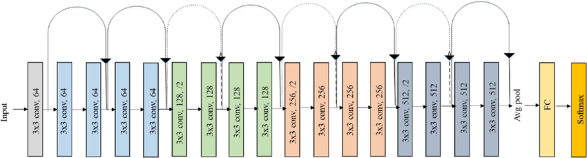
There are no rules regarding the architectures of CNNs, except that they contain convolution and activation layers. In ClinicaDL, other layers such as pooling, batch normalization, dropout and fully-connected layers are also used. The default CNN used for classification in ClinicaDL is Conv5_FC3 which is a convolutional neural network with 5 convolution and 3 fully-connected layer, but in this notebook we will use the resnet18:

resnet18 architecture — *Example of a CNN architecture*

2D slice-level tensor extraction with the `prepare-data` pipeline#

Before starting, we need to obtain the files suited for the training phase. This pipeline prepares images generated by Clinica to be used with the PyTorch deep learning library (Paszke et al., 2019). Four types of tensors are proposed: 3D images, 3D patches, 3D ROI or 2D slices.

The pipeline selects the preprocessed images, extract the “tensors”, and write them as output files for the entire images, for each slice, for each roi or for each patch.

You need to run the following command line:

clinicadl prepare-data {image/patch/roi/slice} <caps_directory> <modality>

where:

caps_directory is the folder in a CAPS hierarchy containing the images corresponding to the modality asked,
modality is the name of the preprocessing performed on the original images (e.g. t1-linear). You can choose custom if you want to get a tensor from a custom filename.

When using patch or slice extraction, default values were set according to Wen et al., 2020

Output files are stored into a new folder (inside the CAPS) and follows a structure like this:

deeplearning_prepare_data
├── image_based
│   └── t1_linear
│       └── sub-<participant_label>_ses-<session_label>_space-MNI152NLin2009cSym_desc-Crop_res-1x1x1_T1w.pt
├── slice_based
│   └── t1_linear
│       ├── sub-<participant_label>_ses-<session_label>_space-MNI152NLin2009cSym_desc-Crop_res-1x1x1_axis-axi_channel-rgb_slice-0_T1w.pt
│       ├── sub-<participant_label>_ses-<session_label>_space-MNI152NLin2009cSym_desc-Crop_res-1x1x1_axis-axi_channel-rgb_slice-1_T1w.pt
│       ├── ...
│       └── sub-<participant_label>_ses-<session_label>_space-MNI152NLin2009cSym_desc-Crop_res-1x1x1_axis-axi_channel-rgb_slice-N_T1w.pt
├── patch_based
│   └── pet-linear
│       ├── sub-<participant_label>_ses-<session_label>_space-MNI152NLin2009cSym_desc-Crop_res-1x1x1_axis-axi_channel-rgb_patch-0_T1w.pt
│       ├── sub-<participant_label>_ses-<session_label>_space-MNI152NLin2009cSym_desc-Crop_res-1x1x1_axis-axi_channel-rgb_patch-1_T1w.pt
│       ├── ...
│       └── sub-<participant_label>_ses-<session_label>_space-MNI152NLin2009cSym_desc-Crop_res-1x1x1_axis-axi_channel-rgb_patch-N_T1w.pt
└── roi_based
    └── t1_linear
        └── sub-<participant_label>_ses-<session_label>_space-MNI152NLin2009cSym_desc-Crop_res-1x1x1_T1w.pt

In short, there is a folder for each feature (image, slice, roi or patch) and inside the numbered tensor files with the corresponding feature. Files are saved with the .pt extension and contains tensors in PyTorch format. A JSON file is also stored in the CAPS hierarchy under the tensor_extraction folder:

CAPS_DIRECTORY
└── tensor_extraction
        └── <extract_json>.json

This file is compulsory to run the train command. It provides all the details of the processing performed by the prepare-data command that will be necessary when reading the tensors.

Warning

The default behavior of the pipeline is to only extract images, even if another extraction method is specified. However, all the options will be saved in the preprocessing JSON file and then, the extraction is done when data is loaded during the training. If you want to save the extracted method tensors in the CAPS, you have to add the --save-features flag.

ClinicaDL is able to extract patches/roi or slices on-the-fly (from one single file) when running training or inference tasks. The downside of this approach is that, depending on the size of your dataset, you have to make sure that you have enough memory resources in your GPU card to host the full images/tensors for all your data.

If the memory size of the GPU card you use is too small, we suggest that you extract the patches and/or the slices using the proper tensor_format option of the command described above.

Before starting#

If you failed to obtain the preprocessing using the t1-linear pipeline, please uncomment the next cell. You can extract tensors from this CAPS, but for the training part you will need a bigger dataset.

!curl -k https://aramislab.paris.inria.fr/clinicadl/files/handbook_2023/data_oasis/CAPS_example.tar.gz -o oasisCaps.tar.gz
!tar xf oasisCaps.tar.gz

If you have already downloaded the full dataset and converted it to CAPS, you can give the path to the dataset directory by changing the CAPS path. If not, just run it as written but the results will not be relevant.

To perform the feature extraction for our dataset, run the following cell:

!clinicadl prepare-data slice data_oasis/CAPS_example t1-linear --extract_json slice_classification_t1

At the end of this command, a new directory named deeplearning_prepare_data is created inside each subject/session of the CAPS structure. We can easily verify. If you failed to obtain the extracted tensors please uncomment the next cell.

!curl -k https://aramislab.paris.inria.fr/clinicadl/files/handbook_2023/data_oasis/CAPS_example_prepared.tar.gz -o oasisCaps.tar.gz
!tar xf oasisCaps.tar.gz

!tree -L 3 data_oasis/CAPS_example/subjects/sub-OASIS10*/ses-M000/deeplearning_prepare_data/

Train your own models#

Before starting#

Warning

If you do not have access to a GPU, training the CNN may take too much time. However, you can execute this notebook on Colab to run it on a GPU.

If you already know the models implemented in clinicadl, you can directly jump to this section to implement your own custom experiment!

import torch

# Check if a GPU is available
print('GPU is available: ', torch.cuda.is_available())

Data used for training#

Because they are time-costly, the preprocessing steps presented in the beginning of this tutorial were only executed on a subset of OASIS-1, but obviously two participants are insufficient to train a network! To obtain more meaningful results, you should retrieve the whole OASIS-1 dataset and run the training based on the labels and splits obtained in the previous section.
Of course, you can use another dataset, on which you will also have to perform labels extraction and data splitting.

`train classification`#

This functionality mainly relies on the PyTorch deep learning library [Paszke et al., 2019].

Different tasks can be learnt by a network: classification, reconstruction and regression. In this notebook, we focus on the classification task.

CNN and 2D slice-level for classification#

An advantage of the 2D slice-level approach is that existing CNNs which had huge success for natural image classification, e.g. ResNet (He et al., 2016) and VGGNet (Simonyan and Zisserman, 2014), can be easily borrowed and used in a transfer learning fashion. Other advantages are the increased number of training samples as many slices can be extracted from a single 3D image, and a lower memory usage compared to using the full MR image as input. This paradigm can be divided into two different frameworks:

single-CNN: one CNN is trained on all slice locations.
multi-CNN: one CNN is trained per slice location.

For multi-CNN the sample size is smaller (equivalent to image level framework), however the CNNs may be more accurate as they are specialized for one slice location.

During training, gradient updates are done based on the loss computed at the slice level. Final performance metric are computed at the subject level by combining the outputs of the slices of the same subject.

Prerequisites#

You need to execute clinicadl tsvtools get-labels and clinicadl tsvtools {split|kfold} commands prior to running this task to have the correct TSV file organization. Moreover, there should be a CAPS, obtained running the preprocessing pipeline wanted.

Running the task#

The training task can be run with the following command line:

clinicadl train classification [OPTIONS] CAPS_DIRECTORY PREPROCESSING_JSON \
                TSV_DIRECTORY OUTPUT_MAPS_DIRECTORY

where mandatory arguments are:

CAPS_DIRECTORY (Path) is the input folder containing the neuroimaging data in a CAPS hierarchy. In case of multi-cohort training, must be a path to a TSV file.
PREPROCESSING_JSON (str) is the name of the preprocessing json file stored in the CAPS_DIRECTORY that corresponds to the clinicadl extract output. This will be used to load the correct tensor inputs with the wanted preprocessing.
TSV_DIRECTORY (Path) is the input folder of a TSV file tree generated by clinicadl tsvtools {split|kfold}. In case of multi-cohort training, must be a path to a TSV file.
OUTPUT_MAPS_DIRECTORY (Path) is the folder where the results are stored.

The training can be configured through a TOML configuration file or by using the command line options. If you have a TOML configuration file you can use the following option to load it:

--config_file (Path) is the path to a TOML configuration file. This file contains the value for the options that you want to specify (to avoid too long command line).

If an option is specified twice (in the configuration file and, as an option, in the command line) then the values specified in the command line will override the values of the configuration file.

A few options depend on the classification task:

--label (str) is the name of the column containing the label for the classification task. It must be a categorical variable, but may be of any type. Default: diagnosis.
--selection_metrics (str) are metrics used to select networks according to the best validation performance. Default: loss.
--selection_threshold (float) is a selection threshold used for soft-voting. It is only taken into account if several images are extracted from the same original 3D image (i.e. num_networks > 1). Default: 0.
--loss (str) is the name of the loss used to optimize the classification task. Must correspond to a PyTorch class. Default: CrossEntropyLoss.

Note

Users can also set themselves the label_code parameter, but only from the configuration file. This parameter allows to choose which name as written in the label column is associated with which node value (designated by the corresponding integer). This way several names may be associated with the same node.

The default label for the classification task is diagnosis but as long as it is a categorical variable, it can be of any type.

The next cell train a resnet18 to classify 2D slices of t1-linear MRI by diagnosis (AD or CN). Please note that the purpose of this notebook is not to fully train a network because we don’t have enough data. The objective is to understand how ClinicaDL works and make inferences using pretrained models in the next section.

# 2D-slice single-CNN training
!clinicadl train classification -h
!clinicadl train classification data_oasis/CAPS_example slice_classification_t1 data_oasis/split/4_fold/ data_oasis/maps_classification_2D_slice_resnet18 --n_splits 4 --architecture resnet18 

# 2D-slice multi-CNN training
!clinicadl train classification data_oasis/CAPS_example slice_classification_t1 data_oasis/split/4_fold/ data_oasis/maps_classification_2D_slice_multi --n_splits 4 --architecture resnet18 --multi_network

The clinicadl train command outputs a MAPS structure in which there are only two data groups: train and validation. A MAPS folder contains all the elements obtained during the training and other post-processing procedures applied to a particular deep learning framework. The hierarchy is organized according to the fold, selection metric and data group used.

An example of a MAPS structure is given below:

<maps_directory>
├── environment.txt
├── split-0
│       ├── best-loss
│       │       ├── model.pth.tar
│       │       ├── train
│       │       │       ├── description.log
│       │       │       ├── train_image_level_metrics.tsv
│       │       │       └── train_image_level_prediction.tsv
│       │       └── validation
│       │               ├── description.log
│       │               ├── validation_image_level_metrics.tsv
│       │               └── validation_image_level_prediction.tsv
│       └── training_logs
│               ├── tensorboard
│               │       ├── train
│               │       └── validation
│               └── training.tsv
├── groups
│       ├── train
│       │       ├── split-0
│       │       │       ├── data.tsv
│       │       │       └── maps.json
│       │       └── split-1
│       │               ├── data.tsv
│       │               └── maps.json
│       ├── train+validation.tsv
│       └── validation
│               ├── split-0
│               │       ├── data.tsv
│               │       └── maps.json
│               └── split-1
│                       ├── data.tsv
│                       └── maps.json
└── maps.json

You can find more information about MAPS structure on our documentation

Inference using pretrained models#

(If you failed to train the model please uncomment the next cell)

!curl -k https://aramislab.paris.inria.fr/clinicadl/files/handbook_2023/data_oasis/maps_classification_2D_slice_multi.tar.gz -o maps_classification_2D_slice_multi.tar.gz
!tar xf maps_classification_2D_slice_multi.tar.gz

!curl -k https://aramislab.paris.inria.fr/clinicadl/files/handbook_2023/data_oasis/maps_classification_2D_slice_resnet.tar.gz -o maps_classification_2D_slice_resnet.tar.gz
!tar xf maps_classification_2D_slice_resnet.tar.gz

If you failed to train the model, you also need to download the TSV files with the list of participants for each split used for the training because clinicadl tsvtools split and clinicadl tsvtools kfold commands randomly split data so you can have data leakage error (see previous notebook for more information about data leakage).

!curl -k https://aramislab.paris.inria.fr/clinicadl/files/handbook_2023/data_oasis/split.tar.gz -o training_split.tar.gz
!tar xf training_split.tar.gz

The predict functionality performs individual prediction and metrics computation on a set of data using models trained with clinicadl train or clinicadl random-search tasks. It can also use any pretrained models if they are structured like a MAPS

Running the task#

This task can be run with the following command line:

  clinicadl predict [OPTIONS] INPUT_MAPS_DIRECTORY DATA_GROUP

where:

INPUT_MAPS_DIRECTORY (Path) is the path to the MAPS of the pretrained model.
DATA_GROUP (str) is the name of the data group used for the prediction.

Warning

For ClinicaDL, a data group is linked to a list of participants / sessions and a CAPS directory. When performing a prediction, interpretation or tensor serialization the user must give a data group. If this data group does not exist, the user MUST give a caps_directory and a participants_tsv. If this data group already exists, the user MUST not give any caps_directory or participants_tsv, or set overwrite to True.

If you want to add optional argument you can check the documentation.

!clinicadl predict -h
!clinicadl predict data_oasis/maps_classification_2D_slice_resnet18 'test-Oasis2' --participants_tsv ./data_oasis/split/test_baseline.tsv --caps_directory data_oasis/CAPS_example

!clinicadl predict data_oasis/maps_classification_2D_slice_multi 'test-Oasis' --participants_tsv ./data_oasis/split/test_baseline.tsv --caps_directory data_oasis/CAPS_example

Results are stored in the MAPS of path model_path, according to the following file system:

model_path>
    ├── split-0  
    ├── ...  
    └── split-<i>
        └── best-<metric>
                └── <data_group>
                    ├── description.log
                    ├── <prefix>_image_level_metrics.tsv
                    ├── <prefix>_image_level_prediction.tsv
                    ├── <prefix>_slice_level_metrics.tsv
                    └── <prefix>_slice_level_prediction.tsv

clinica predict produces a file containing different metrics (accuracy, balanced accuracy, etc.) for the current dataset. It can be displayed by running the next cell:

import pandas as pd
metrics = pd.read_csv("data_oasis/maps_classification_2D_slice_resnet18/split-0/best-loss/test-Oasis/test-OASIS_slice_level_metrics.tsv", sep="\t")
metrics.head()

Deep Learning Classification from brain MRI

Classification with a CNN on 2D slice

Contents

Classification with a CNN on 2D slice#

2D slice-level tensor extraction with the `prepare-data` pipeline#

Before starting#

Train your own models#

Before starting#

Data used for training#

`train classification`#

CNN and 2D slice-level for classification#

Prerequisites#

Running the task#

Inference using pretrained models#

Running the task#

Deep Learning Classification from brain MRI

Classification with a CNN on 2D slice

Contents

Classification with a CNN on 2D slice#

2D slice-level tensor extraction with the prepare-data pipeline#

Before starting#

Train your own models#

Before starting#

Data used for training#

train classification#

CNN and 2D slice-level for classification#

Prerequisites#

Running the task#

Inference using pretrained models#

Running the task#

2D slice-level tensor extraction with the `prepare-data` pipeline#

`train classification`#