Deep learning: application to neuroimaging

Deep learning is an ill-defined term that may refer to many different concepts. In this notebook, deep learning designate methods used to optimize a network that executes a task whose success is quantified by a loss function. This optimization or learning process is based on a dataset, whose samples are used to optimize the parameters of the network.

Deep learning networks are a succession of functions (called layers) which transform their inputs in outputs (called feature maps). There are two types of layers:

• Layers including learnable parameters that will be updated to improve the loss (for example convolutions).

• Layers with fixed behavior during the whole training process (for example pooling or activation functions).

Indeed, some characteristics are not modified during the training of the networks. These components are fixed prior to training according to hyperparameters, such as the number of layers or intrinsic characteristics of layers. One of the main difficulties of deep learning is often not to train the networks, but to find good hyperparameters that will be adapted to the task and the dataset. This problem gave birth to a research field called Neural Architecture Search (NAS). A basic method of NAS, the random search, is the theme of one of the last notebooks.

Why deep ?

Originally the term deep was used to differentiate shallow networks, with only one layer, from those with two layers are more. Today the distinction is not really useful anymore as most of the networks have way more than two layers!

Common network layers

In a deep learning network every function is called a layer though the operations layers perform are very different. You will find below a summary of the layers composing the architectures used in the following sections of this tutorial.

Convolution

The aim of a convolution layer is to learn a set of filters (or kernels) which capture useful patterns in the data distribution. These filters parse the input feature map using translations:

A convolution layer captures local patterns that are limited to the size of its filters. However, a succession of several convolutions allows increasing the receptive field, i.e. the size of the region used in the input image to compute one value of the output feature map. In this way, the first layer of the network will capture local patterns in the image (edges, homogeneous regions) and the next one will assemble these patterns to form more and more complex patterns (gyri and sulci, then regions of the brain).

Batch normalization

This layer learns to normalize feature maps according to (Ioffe & Szegedy, 2015). Adding this layer to a network may accelerate the training procedure.

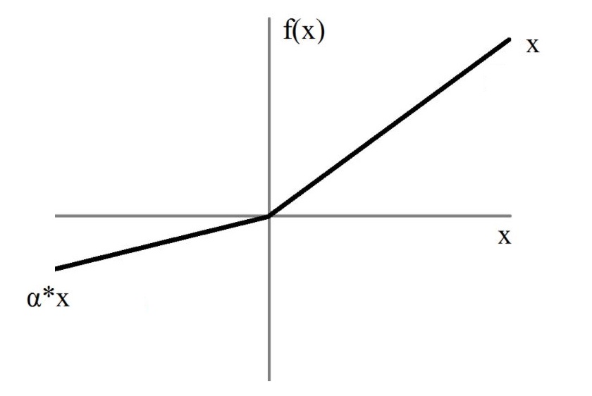
Activation function (Leaky ReLU)

To introduce non-linearity in the model, an activation function is introduced after the convolutions and fully-connected layers. Without activation functions, the network would only learn linear combinations!

Many activation functions have been proposed to solve deep learning problems. In the architectures implemented in clinicadl the activation function is Leaky ReLU:

Pooling function

Pooling layers reduce the size of their input feature maps. Their structure is very similar to the convolutional layer: a kernel with a defined size and stride is passing through the input. However there are no learnable parameters in this layer, the kernel outputting the maximum value of the part of the feature map it covers.

Here is an example in 2D of the standard layer of pytorch nn.MaxPool2d:

The last column may not be used depending on the size of the kernel/input and stride value. To avoid this, pooling layers with adaptive padding were implemented in clinicadl to exploit information from the whole feature map.

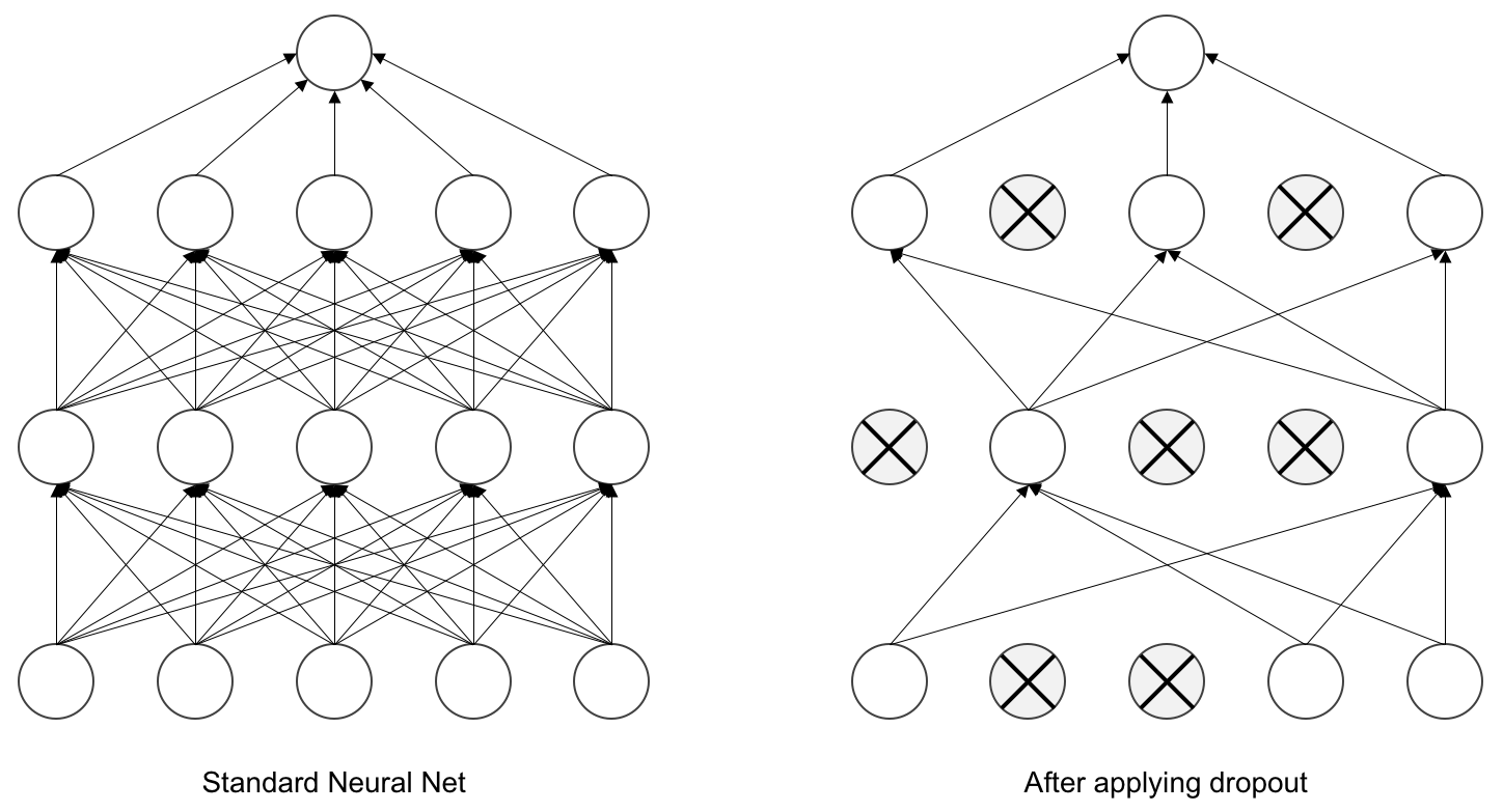
Dropout

Proposed by (Srivastava et al., 2014), dropout layers literally drop out a fixed proportion of the input values (i.e. replace their value by 0). This behavior is enabled during training to limit overfitting, then it is disabled during evaluation to obtain the best possible prediction.

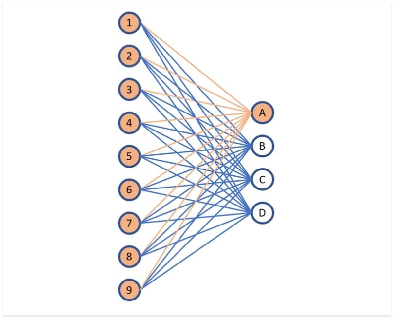
Fully-connected

Contrary to convolutions in which relationships between values are studied locally, fully-connected layers look for a global linear combination between all the input values (hence the term fully-connected). In convolutional neural networks they are often used at the end of the architecture to reduce the final feature maps to a number of nodes equal to the number of classes in the dataset.

Tasks & architectures

Deep learning methods have been used to learn many different tasks such as classification, dimension reduction, data synthesis… In this notebook we focus on the three tasks that we can do with clinicaDL :

• classification of 2D slices using convolutional neural networks (notebook);

• regression on 3D images using convolutional neural network (notebook);

• reconstruction of 3D patches or region of interest using autoencoder (notebook).

To successfully learn a task, a network needs to analyze a large number of labeled samples. In neuroimaging, these samples are costly to acquire and thus their number is limited. However, when trained on small samples, due to the large number of learnt parameters, deep learning models tend to easily overfit.

Overfitting

Overfitting in neuroimaging refers to a situation where a neural network model is trained too well on the training data, resulting in poor performance on new, unseen data. In other words, the model has *memorized the training data instead of learning the underlying patterns and relationships and it can result in poor generalization of the model, where it performs well on the training data but poorly on new data.

Overfitting can be detected by monitoring the training and validation accuracy of the model. If the training accuracy continues to improve while the validation accuracy remains stagnant or decreases, it is a sign of overfitting. Different strategies have been developed to alleviate overfitting. These strategies include dropout, data augmentation or adding a weight decay in the optimizer. Another technique seen in this notebook consists in transferring weights learnt by an autoencoder. Indeed this network can learn patterns representative of the dataset in a self-supervised manner, hence it does not need labels and can be trained on all samples available.