Perfom classification using pretrained models¶

This notebook shows how to perform classification on preprocessed data using pretrained models described in (Wen et al, 2020).

Structure of the pretrained models¶

All the pretrained model folders are organized as follows:

results
├── commandline.json
├── fold-0
├── ...
└── fold-4
    ├── models
    │      └── best_balanced_accuracy
    │          └── model_best.pth.tar
    └── cnn_classification
           └── best_balanced_accuracy
               └── validation_{patch|roi|slice}_level_prediction.tsv

This file system is a part of the output of clinicadl train and clinicadl classify relies on three files:

commandline.json contains all the options that were entered for training (type of input, architecture, preprocessing...).
model_best.pth.tar corresponds to the model selected when the best validation balanced accuracy was obtained.
validation_{patch|roi|slice}_level_prediction.tsv is specific to patch, roi and slice frameworks and is necessary to perform soft-voting and find the label at the image level in unbiased way. Weighting the patches based on their performance of input data would bias the result as the classification framework would exploit knowledge of the test data.

Tip:

You can use your own previuolsy trained model (if you have used PyTorch for that). Indeed, PyTorch stores model weights in a file with extension pth.tar. You can place this file into the models folder and try to follow the same structure that is described above. You also need to fill a commandline.json file with all the parameters used during the training (see ClinicaDL documentation) for further info.

Soft voting:

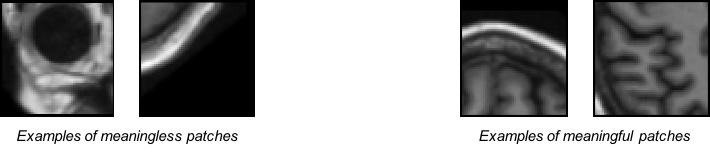
For classification tasks that take as input a part of the MRI volume (patch, roi or slice), an ensemble operation is needed to obtain the label at the image level.

For example, size and stride of 50 voxels on linear preprocessing leads to the classification of 36 patches, but they are not all equally meaningful. Patches that are in the corners of the image are mainly composed of background and skull and may be misleading, whereas patches within the brain may be more useful.

Then the image-level probability of AD p^AD will be:

$$ p^{AD} = {\sum_{i=0}^{35} bacc_i * p_i^{AD}}.$$ where:

p_i^AD is the probability of AD for patch i
bacc_i is the validation balanced accuracy for patch i

Download the pretrained models¶

Warning

Warning: For the sake of the demonstration, this tutorial uses truncated versions of the models, containing only the first fold.

In this notebook, we propose to use 4 specific models , all of them where trained to predict the classification task AD vs CN. (The experiment corresponding to the pretrained model in eTable 4 of the paper mentioned above is shown below):

3D image-level model, pretrained with the baseline data and initialized with an autoencoder (cf. exp. 3).
3D ROI-based model, pretrained with the baseline data and initialized with an autoencoder (cf. exp. 8).
3D patch-level model, multi-cnn, pretrained with the baseline data and initialized with an autoencoder (cf. exp. 14).
2D slice-level model, pretrained with the baseline data and initialized with an autoencoder (cf. exp. 18).

Commands in the next code cell will automatically download and uncompress these models.

# Download here the pretrained models stored online
# Model 1
!curl -k https://aramislab.paris.inria.fr/clinicadl/files/models/v0.2.0/model_exp3_splits_1.tar.gz  -o model_exp3_splits_1.tar.gz
!tar xf model_exp3_splits_1.tar.gz

# Model 2
!curl -k https://aramislab.paris.inria.fr/clinicadl/files/models/v0.2.0/model_exp8_splits_1.tar.gz  -o model_exp8_splits_1.tar.gz
!tar xf model_exp8_splits_1.tar.gz

# Model 3
!curl -k https://aramislab.paris.inria.fr/clinicadl/files/models/v0.2.0/model_exp14_splits_1.tar.gz  -o model_exp14_splits_1.tar.gz
!tar xf model_exp14_splits_1.tar.gz

# Model 4
!curl -k https://aramislab.paris.inria.fr/clinicadl/files/models/v0.2.0/model_exp18_splits_1.tar.gz  -o model_exp18_splits_1.tar.gz
!tar xf model_exp18_splits_1.tar.gz

Run `clinicadl classify`¶

Running classification on a dataset is extremly simple using clinicadl. In this case, we will continue using the data preprocessed in the previous notebook. The models have been trained exclusively on the ADNI dataset, all the subjects of OASIS-1 can be used to evaluate the model (without risking data leakage).

If you ran the previous notebook, you must have a folder called OasisCaps_example in the current directory (Otherwise uncomment the next cell to download a local version of the necessary folders).

!curl -k https://aramislab.paris.inria.fr/files/data/databases/tuto/OasisCaps2.tar.gz -o OasisCaps2.tar.gz
!tar xf OasisCaps2.tar.gz
!curl -k https://aramislab.paris.inria.fr/files/data/databases/tuto/OasisBids.tar.gz -o OasisBids.tar.gz
!tar xf OasisBids.tar.gz

In the following steps we will classify the images using the pretrained models. The input necessary for clinica classify are:

a CAPS directory (OasisCaps_example),
a tsv file with subjects/sessions to process, containing the diagnosis (participants.tsv),
the path to the pretrained model,
an output prefix for the output file.

Some optional parameters includes:

the possibility of classifying non labeled data (without known diagnosis),
the option to use previously extracted patches/slices.

Warning

If your computer is not equiped with a GPU card add the option -cpu to the command.

First of all, we need to generate a valid tsv file. We use the tool clinica iotools:

!clinica iotools merge-tsv OasisBids_example OasisCaps_example/participants.tsv

Then, we can run the classifier for the image-level model:

# Execute classify on OASIS dataset
# Model 1
!clinicadl classify ./OasisCaps_example ./OasisCaps_example/participants.tsv ./model_exp3_splits_1 'test-Oasis'

The predictions of our classifier for the subjects of this dataset are shown next:

import pandas as pd

predictions = pd.read_csv("./model_exp3_splits_1/fold-0/cnn_classification/best_balanced_accuracy/test-Oasis_image_level_prediction.tsv", sep="\t")
predictions.head()

	participant_id	session_id	true_label	predicted_label
0	sub-OASIS10016	ses-M00	1	1
1	sub-OASIS10109	ses-M00	0	0
2	sub-OASIS10304	ses-M00	1	1
3	sub-OASIS10363	ses-M00	0	0

Note that 0 corresponds to the CN class and 1 to the AD. It is also important to remember that the last two images/subjects performed badly when running the quality check step.

clinica classify also produces a file containing different metrics (accuracy, balanced accuracy, etc.) for the current dataset. It can be displayed by running the next cell:

metrics = pd.read_csv("./model_exp3_splits_1/fold-0/cnn_classification/best_balanced_accuracy/test-Oasis_image_level_metrics.tsv", sep="\t")
metrics.head()

	accuracy	balanced_accuracy	sensitivity	specificity	ppv	npv	total_loss	total_kl_loss	image_id
0	1.0	1.0	1.0	1.0	1.0	1.0	1.068584	0	NaN

In the same way, we can process the dataset with all the other models:

# Model 2 3D ROI-based model
!clinicadl classify ./OasisCaps_example ./OasisCaps_example/participants.tsv ./model_exp8_splits_1 'test-Oasis'

predictions = pd.read_csv("./model_exp8_splits_1/fold-0/cnn_classification/best_balanced_accuracy/test-Oasis_image_level_prediction.tsv", sep="\t")
predictions.head()

# Model 3 3D patch-level model
!clinicadl classify ./OasisCaps_example ./OasisCaps_example/participants.tsv ./model_exp14_splits_1 'test-Oasis'

predictions = pd.read_csv("./model_exp14_splits_1/fold-0/cnn_classification/best_balanced_accuracy/test-Oasis_image_level_prediction.tsv", sep="\t")
predictions.head()

# Model 4 2D slice-level model
!clinicadl classify ./OasisCaps_example ./OasisCaps_example/participants.tsv ./model_exp18_splits_1 'test-Oasis'

predictions = pd.read_csv("./model_exp18_splits_1/fold-0/cnn_classification/best_balanced_accuracy/test-Oasis_image_level_prediction.tsv", sep="\t")
predictions.head()

Deep learning classification from brain MRI

Perfom classification using pretrained models¶

Structure of the pretrained models¶

Download the pretrained models¶

Run clinicadl classify¶

Run `clinicadl classify`¶