`pet-surface` - Surface-based processing of PET images¶

This pipeline performs several processing steps for the analysis of PET data on the cortical surface [Marcoux et al., 2018]:

co-registration of PET and T1-weighted MR images;
intensity normalization;
partial volume correction;
robust projection of the PET signal onto the subject’s cortical surface;
spatial normalization to a template;
atlas statistics.

This pipeline relies mainly on tools from FreeSurfer and PETPVC [Thomas et al., 2016].

Clinica & BIDS specifications for PET modality

Since Clinica v0.6, PET data following the official specifications in BIDS version 1.6.0 are now compatible with Clinica. See BIDS page for more information.

Prerequisite¶

You need to have performed the t1-freesurfer pipeline on your T1-weighted MR images.

Dependencies¶

If you only installed the core of Clinica, this pipeline needs the installation of FreeSurfer 6.0, FSL 6.0, and PETPVC 1.2.4 (which depends on ITK 4) on your computer.

In addition, you also need to either install SPM12 and Matlab, or spm standalone.

Running the pipeline¶

The pipeline can be run with the following command line:

clinica run pet-surface [OPTIONS] BIDS_DIRECTORY CAPS_DIRECTORY ACQ_LABEL
                        {pons|cerebellumPons|pons2|cerebellumPons2} PVC_PSF_TSV

where:

BIDS_DIRECTORY is the input folder containing the dataset in a BIDS hierarchy.
CAPS_DIRECTORY acts both as an input folder (where the results of the t1-freesurfer pipeline are stored) and as the output folder containing the results in a CAPS hierarchy.
ACQ_LABEL is the label given to the PET acquisition, specifying the tracer used (trc-<acq_label>).
The reference region is used to perform intensity normalization (i.e. dividing each voxel of the image by the average uptake in this region) resulting in a standardized uptake value ratio (SUVR) map. It can be cerebellumPons or cerebellumPons2 (used for amyloid tracers) or pons or pons2 (used for FDG).
PVC_PSF_TSV is the TSV file containing the psf_x, psf_y and psf_z of the PSF for each PET image. It is expected to be generated by the user. More explanation is given in PET Introduction page.

Info

Since the release of Clinica v0.3.8, the handling of PSF information has changed. In previous versions of Clinica, each BIDS-PET image had to contain a JSON file with the EffectiveResolutionInPlane and EffectiveResolutionAxial fields corresponding to the PSF in mm. EffectiveResolutionInPlane is replaced by both psf_x and psf_y, EffectiveResolutionAxial is replaced by psf_z and the acq_label column has been added. Additionally, the SUVR reference region is now a compulsory argument: it will be easier for you to modify Clinica if you want to add a custom reference region (PET Introduction page). Choose cerebellumPons for amyloid tracers or pons for FDG to have the previous behavior.

Pipeline options:

--reconstruction_method: Select only images based on a specific reconstruction method.
-np: This parameter specifies the number of threads to run in parallel. We recommend using your_number_of_cpu - 1.

Please note that PETPVC is extremely demanding in terms of resources and may cause the pipeline to crash if many subjects happen to be partial volume corrected at the same time (Error : Failed to allocate memory for image). To mitigate this issue, you can do the following:

**1)** Use a working directory when you launch Clinica.

**2)** If the pipeline crashed, just launch again the command (while giving the same working directory).
The whole processing will continue where it left (you can reduce the number of threads to run in parallel the second time).

Note

The arguments common to all Clinica pipelines are described in Interacting with clinica.

Tip

Do not hesitate to type clinica run pet-surface --help to see the full list of parameters.

Known error on macOS

If you are running pet-surface on macOS, we noticed that if the path to the CAPS is too long, the pipeline fails when the gtmseg command from FreeSurfer is executed. This generates crash files with gtmseg in the filename, for instance:

$ nipypecli crash crash-20210404-115414-sheldon.cooper-gtmseg-278e3a57-294f-4121-8a46-9975801f24aa.pklz
[...]
Abort
ERROR: mri_gtmseg --s sub-ADNI011S4105_ses-M000 --usf 2 --o gtmseg.mgz --apas apas+head.mgz --no-subseg-wm --no-keep-cc --no-keep-hypo
gtmseg exited with errors
Standard error:
Saving result to '<caps>/subjects/sub-ADNI011S4105/ses-M000/t1/freesurfer_cross_sectional/sub-ADNI011S4105_ses-M000/tmp/tmpdir.xcerebralseg.50819/tmpdir.fscalc.53505/tmp.mgh' (type = MGH )                       [ ok ]
Saving result to '<caps>/subjects/sub-ADNI011S4105/ses-M000/t1/freesurfer_cross_sectional/sub-ADNI011S4105_ses-M000/tmp/tmpdir.xcerebralseg.50819/tmpdir.fscalc.53727/tmp.mgh' (type = MGH )                       [ ok ]
Saving result to '<caps>/subjects/sub-ADNI011S4105/ses-M000/t1/freesurfer_cross_sectional/sub-ADNI011S4105_ses-M000/tmp/tmpdir.xcerebralseg.50819/tmpdir.fscalc.53946/tmp.mgh' (type = MGH )                       [ ok ]
Return code: 1

This is under investigation (see Issue #119 for details) and will be solved as soon as possible.

Outputs¶

Results are stored in the following folder of the CAPS hierarchy: subjects/<participant_id>/<session_id>/pet/surface

The main output files are (where * stands for <participant_id>_<session_id>):

*_trc-<label>_pet_space-<label>_suvr-<label>_pvc-iy_hemi-<label>_fwhm-<value>_projection.mgh: PET data that can be mapped onto meshes. If the space is fsaverage, it can be mapped either onto the white or pial surface of FsAverage. If the space is native, it can be mapped onto the white or pial surface of the subject’s surface (i.e. {l|r}h.white, {l|r}h.pial files from the t1-freesurfer pipeline).
*_hemi-{left|right}_midcorticalsurface: surface at equal distance between the white matter/gray matter interface and the pial surface (one per hemisphere).
atlas_statistics/*_trc-<label>_pet_space-<label>_pvc-iy_suvr-<label>_statistics.tsv: TSV files summarizing the regional statistics on the labelled atlases (Desikan and Destrieux).

Note

The full list of output files from the pet-surface pipeline can be found in The ClinicA Processed Structure (CAPS) specifications.

FDG PET SUVR projected onto the cortical surface (left hemisphere) for (from left to right) a cognitively normal subject (CN), a patient with Alzheimer’s disease (AD), a patient with semantic variant primary progressive aphasia (svPPA) and a patient with logopenic variant primary progressive aphasia (lvPPA). The first row is the projection in the subject’s space. The second row is the same signal for each subject, but warped to FsAverage after smoothing with a 20 mm Gaussian kernel.

Going further¶

You can use projected PET data to perform group comparison or correlation analysis with the statistics-surface pipeline.
You can use projected PET data to perform classification based on machine learning, as showcased in the AD-ML framework.

Describing this pipeline in your paper¶

Example of paragraph:

These results have been obtained using the pet-surface pipeline of Clinica [Routier et al., 2021; Marcoux et al., 2018]. The subject’s PET image was registered to the T1-weighted MRI using spmregister (FreeSurfer) and intensity normalized using the [pons | pons and cerebellum] from the Pick atlas in MNI space as reference region (registration to MNI space was performed using SPM12). Partial volume correction was then performed using the iterative Yang algorithm implemented in PETPVC [Thomas et al., 2016] with regions obtained from gtmseg (FreeSurfer). Based on the subject’s white surface and cortical thickness, seven surfaces for each hemisphere were computed, ranging from 35% to 65% of the gray matter thickness. The partial volume corrected data were projected onto these meshes and the seven values were averaged, giving more weight to the vertices near the center of the cortex. Finally, the projected PET signal in the subject’s native space was spatially normalized to the standard space of FsAverage (FreeSurfer).

Tip

Easily access the papers cited on this page on Zotero.

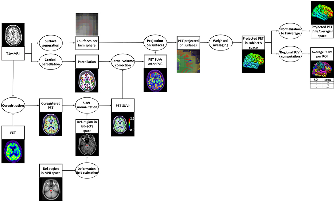
Appendix I: Diagram of the pipeline execution¶

The subject's T1-weighted MRI is coregistered with the PET image and the PET image is intensity normalized using the average uptake in a reference region. In parallel, cortical surfaces and a parcellation are generated from the subject's T1-weighted MRI. The PET image, after partial volume correction performed using the parcellation, is robustly projected onto the cortical surface. Finally, regional mean uptake values are extracted from the projected PET data, and the projected PET signal in the subject's native space is spatially normalized to the standard space of FsAverage.

Appendix II: How to manipulate outputs¶

Outputs of pipeline are composed of two different types of file: surface files and MGH data that are to be overlaid onto a surface.

Surface file¶

Surface files can be read using various software packages. You can open them using freeview (FreeSurfer viewer), with freeview -f /path/to/your/surface/file.

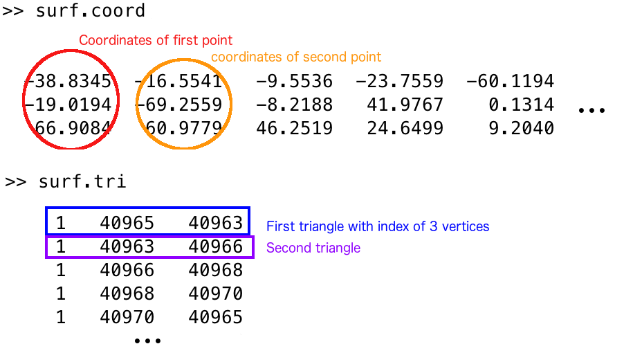
You can also open them in MATLAB, using SurfStat: mysurface = SurfStatReadSurf('/path/to/your/surface/file'). This will give you a structure with fields coord (for coordinates), a list of coordinates for each point of the mesh, and also the field tri (for triangle), a list of triplet for each triangle, each number representing the Nth vertex of the coord list. Below is an example to make things clearer (read with Matlab).

Data files¶

Data files wear the .mgh extension. They are composed of a single vector. These files contain a vector, where the value at the Nth position must be mapped into the Nth vertex of the coord list to be correctly represented. You can access them either in Matlab with the command:

mydata = SurfStatReadData('/path/to/your/file.mgh');

(you will get a single row vector),

or in Python with the nibabel library:

import nibabel
mydata = nibabel.load('/path/to/your/mgh/file')

mydata will then be a MGHImage, more information here. Keep in mind that if you want to manipulate the data vector within this object, you will need to transform it a bit. Indeed, if you do the following:

raw_data = mydata.get_fdata(dtype="float32")
print(raw_data.shape)

The shape of your "raw" vector will probably look like this: (163842, 1, 1). Use the squeeze function from numpy to get a (163842,) shape (documentation here). The reverse operation ((163842,) to a (163842, 1, 1) shape) can be achieved with the atleast_3d function from numpy (documentation here). This may come handy when you need to create a MGHImage from scratch.

Visualization of the results¶

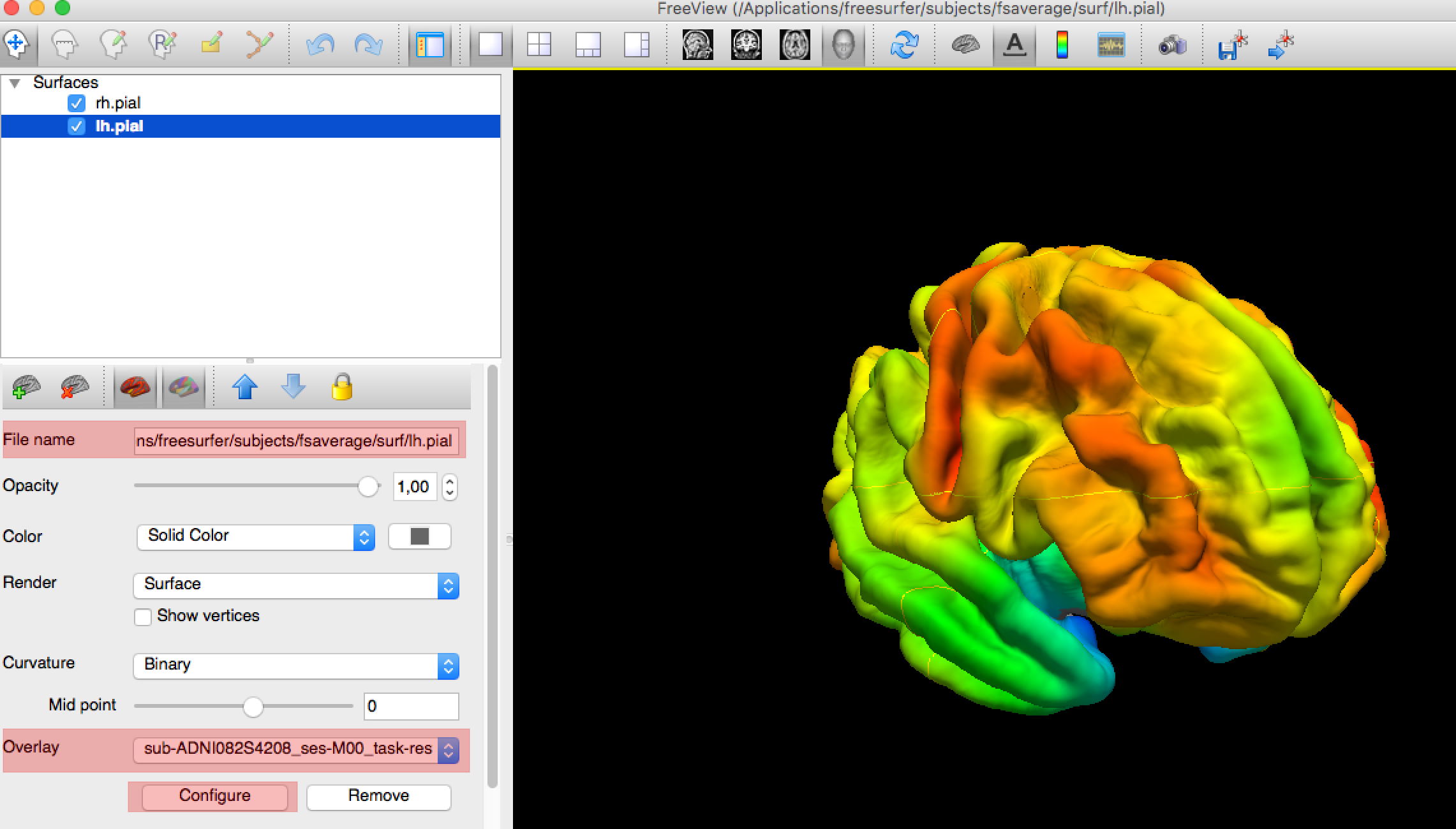
After the execution of the pipeline, you can check the outputs of a subject by running this command (subject moved into FsAverage):

freeview -f $SUBJECTS_DIR/fsaverage/surf/lh.pial:overlay=path/to/your/projected/pet/in/fsaverage/left/hemi \
 -f $SUBJECTS_DIR/fsaverage/surf/rh.pial:overlay=path/to/your/projected/pet/in/fsaverage/right/hemi

But you can also visualize your subject cortical projection directly into his native space:

freeview -f path/to/midcortical/surface/left:overlay=path/to/your/projected/pet/in/nativespace/left/hemi \
 -f path/to/midcortical/surface/right:overlay=path/to/your/projected/pet/in/nativespace/right/hemi

You will need to adjust the colormap using the Configure button in the left panel, just below the Overlay section.

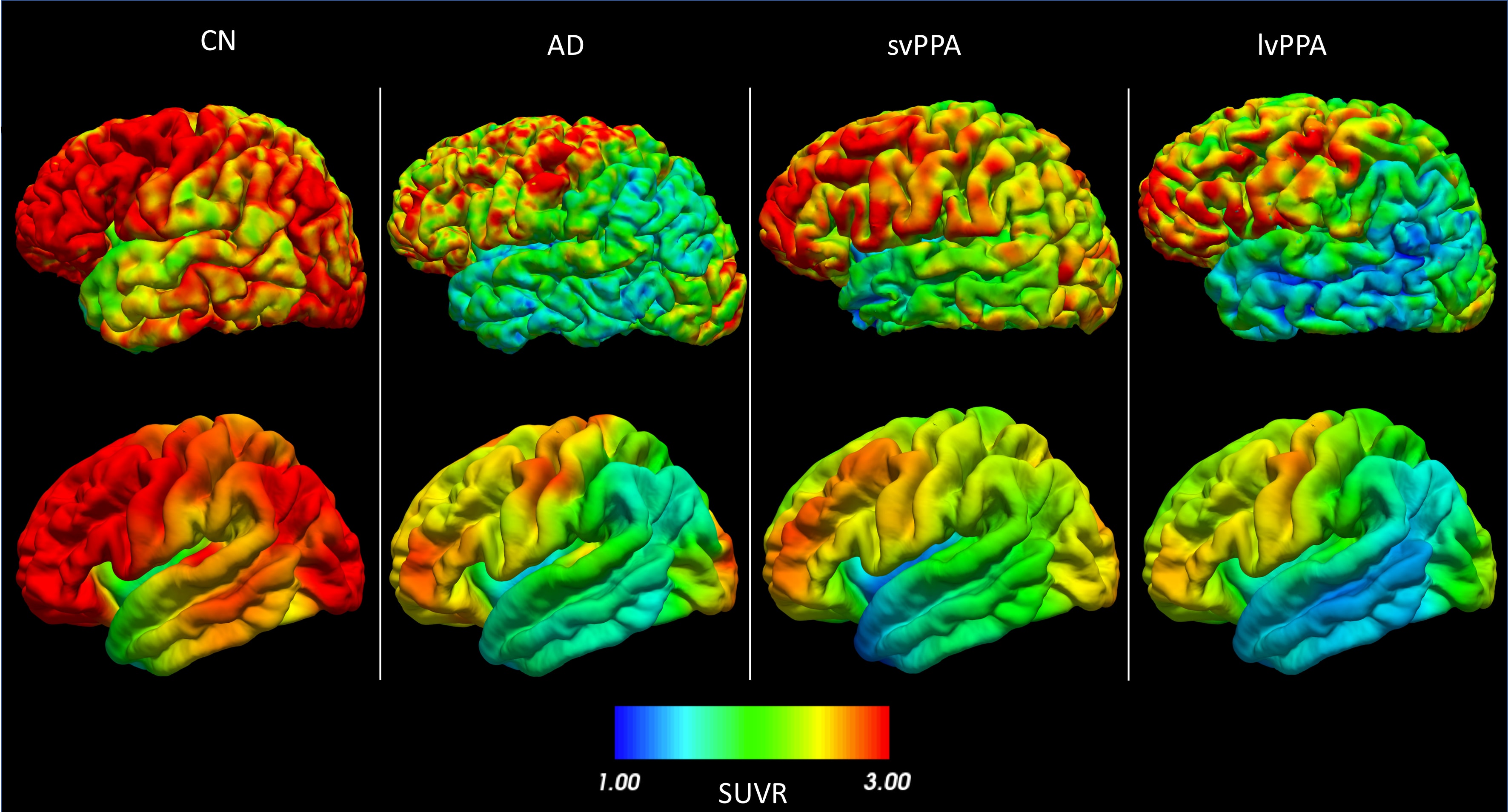
You can also visualize your surface using the SurfStat tool. Once the SurfStat installation folder is added to your MATLAB path, you can display your surfaces with the following commands:

mydata = SurfStatReadData({'/path/to/left/data', '/path/to/right/data'});
mysurfaces = SurfStatReadSurf({'/path/to/left/surface', '/path/to/right/surface'});
figure, SurfStatViewData(mydata, mysurfaces, 'Title of figure');

You will obtain the following figure:

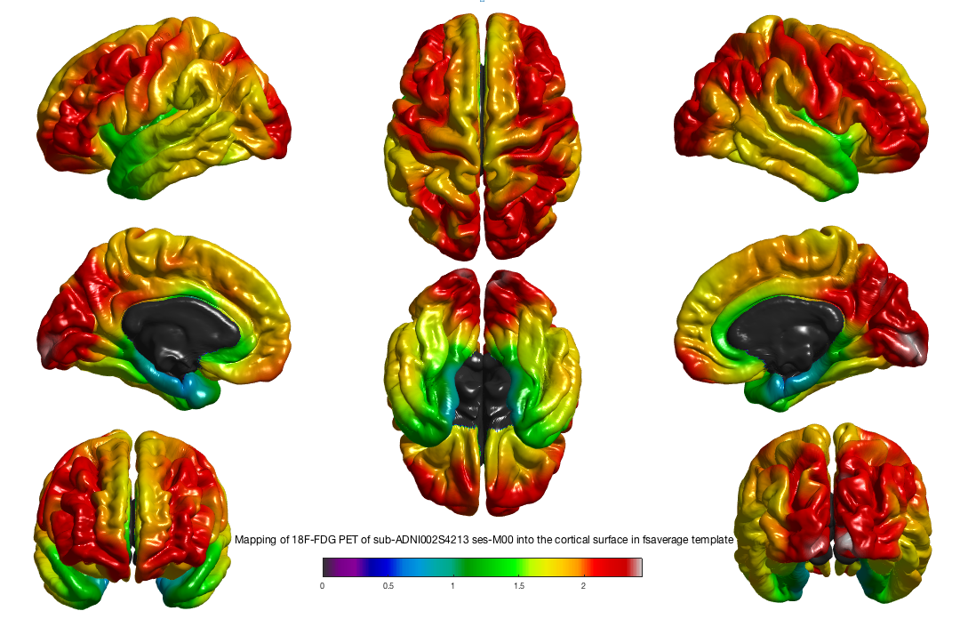
Contact us !¶

Check for past answers on Clinica Google Group
Start a discussion on GitHub
Report an issue on Github

pet-surface - Surface-based processing of PET images¶