
0. Classification of Alzheimer’s disease diagnosis
Contenu
Note
If running in Colab, think of changing the runtime type before starting, in order to have access to GPU ressources: Runtime->Change Runtime Type, then chose GPU for hardware accelerator.
0. Classification of Alzheimer’s disease diagnosis
The goal of this lab session is to train a network that will perform a binary classification between control participants and patients that are affected by Alzheimer’s disease. The input of the network is a neuroimaging modality: the T1 weighted MRI. In this project we use the Pytorch library.
import torch
import numpy as np
import pandas as pd
from torch import nn
from time import time
from os import path
from torchvision import transforms
import random
from copy import deepcopy
Database
In this session we use the images from a public research project: OASIS-1. Two labels exist in this dataset:
CN (Cognitively Normal) for healthy participants.
AD (Alzheimer’s Disease) for patients affected by Alzheimer’s disease.
The original images were preprocessed using Clinica: a software platform for clinical neuroimaging studies. Preprocessed images and other files are distributed in a tarball, run the following commands to download and extract them.
! wget --no-check-certificate --show-progress https://aramislab.paris.inria.fr/files/data/databases/DL4MI/OASIS-1-dataset_pt_new.tar.gz
--2022-01-20 18:25:26--  https://aramislab.paris.inria.fr/files/data/databases/DL4MI/OASIS-1-dataset_pt_new.tar.gz
Résolution de aramislab.paris.inria.fr (aramislab.paris.inria.fr)… 128.93.101.229
Connexion à aramislab.paris.inria.fr (aramislab.paris.inria.fr)|128.93.101.229|:443… connecté.
Avertissement : impossible de vérifier l’attribut aramislab.paris.inria.fr du certificat, émis par «CN=TERENA SSL CA 3,O=TERENA,L=Amsterdam,ST=Noord-Holland,C=NL» :
  Impossible de vérifier localement l’autorité de l’émetteur.
requête HTTP transmise, en attente de la réponse… 200 OK
Taille : 1387416064 (1,3G) [application/octet-stream]
Enregistre : «OASIS-1-dataset_pt_new.tar.gz»


          OASIS-1-d   0%[                    ]       0  --.-KB/s
OASIS-1-da 1%[ ] 21,29M 102MB/s
OASIS-1-dat 3%[ ] 44,66M 109MB/s
OASIS-1-data 5%[> ] 67,02M 110MB/s
OASIS-1-datas 6%[> ] 88,68M 110MB/s
OASIS-1-datase 8%[> ] 111,01M 110MB/s
OASIS-1-dataset 10%[=> ] 133,37M 110MB/s
OASIS-1-dataset_ 11%[=> ] 151,55M 108MB/s
OASIS-1-dataset_p 12%[=> ] 169,51M 105MB/s
OASIS-1-dataset_pt 14%[=> ] 187,38M 104MB/s
OASIS-1-dataset_pt_ 15%[==> ] 204,07M 102MB/s
ASIS-1-dataset_pt_n 16%[==> ] 220,66M 99,8MB/s
SIS-1-dataset_pt_ne 17%[==> ] 226,04M 80,6MB/s
IS-1-dataset_pt_new 18%[==> ] 242,96M 80,8MB/s tps 13s
S-1-dataset_pt_new. 19%[==> ] 259,84M 81,1MB/s tps 13s
-1-dataset_pt_new.t 20%[===> ] 276,67M 81,3MB/s tps 13s
1-dataset_pt_new.ta 22%[===> ] 293,48M 80,4MB/s tps 13s
-dataset_pt_new.tar 23%[===> ] 310,37M 79,3MB/s tps 13s
dataset_pt_new.tar. 24%[===> ] 325,92M 77,8MB/s tps 12s
ataset_pt_new.tar.g 26%[====> ] 344,58M 75,8MB/s tps 12s
taset_pt_new.tar.gz 27%[====> ] 360,82M 74,7MB/s tps 12s
aset_pt_new.tar.gz 28%[====> ] 377,30M 73,6MB/s tps 12s
set_pt_new.tar.gz 29%[====> ] 394,63M 71,9MB/s tps 12s
et_pt_new.tar.gz 31%[=====> ] 411,88M 71,8MB/s tps 11s
t_pt_new.tar.gz 32%[=====> ] 429,30M 72,0MB/s tps 11s
_pt_new.tar.gz 33%[=====> ] 445,80M 71,2MB/s tps 11s
pt_new.tar.gz 35%[======> ] 463,79M 71,9MB/s tps 11s
t_new.tar.gz 36%[======> ] 480,77M 72,5MB/s tps 11s
_new.tar.gz 37%[======> ] 497,13M 84,6MB/s tps 10s
new.tar.gz 38%[======> ] 513,43M 84,2MB/s tps 10s
ew.tar.gz 40%[=======> ] 529,69M 84,2MB/s tps 10s
w.tar.gz 41%[=======> ] 546,10M 84,2MB/s tps 10s
.tar.gz 42%[=======> ] 562,77M 84,1MB/s tps 10s
tar.gz 43%[=======> ] 579,43M 84,4MB/s tps 9s
ar.gz 44%[=======> ] 595,15M 83,6MB/s tps 9s
r.gz 46%[========> ] 611,57M 83,5MB/s tps 9s
.gz 47%[========> ] 631,33M 84,6MB/s tps 9s
gz 49%[========> ] 650,57M 85,4MB/s tps 9s
z 50%[=========> ] 667,07M 85,0MB/s tps 8s
51%[=========> ] 685,30M 85,2MB/s tps 8s
O 53%[=========> ] 703,44M 85,7MB/s tps 8s
OA 54%[=========> ] 721,88M 85,9MB/s tps 8s
OAS 55%[==========> ] 740,10M 86,3MB/s tps 8s
OASI 57%[==========> ] 758,43M 86,8MB/s tps 7s
OASIS 58%[==========> ] 776,96M 87,5MB/s tps 7s
OASIS- 59%[==========> ] 793,52M 87,8MB/s tps 7s
OASIS-1 61%[===========> ] 810,18M 87,6MB/s tps 7s
OASIS-1- 62%[===========> ] 827,22M 88,0MB/s tps 7s
OASIS-1-d 63%[===========> ] 845,51M 88,6MB/s tps 6s
OASIS-1-da 65%[============> ] 864,51M 89,4MB/s tps 6s
OASIS-1-dat 66%[============> ] 881,94M 90,0MB/s tps 6s
OASIS-1-data 67%[============> ] 898,32M 88,9MB/s tps 6s
OASIS-1-datas 69%[============> ] 914,74M 88,1MB/s tps 6s
OASIS-1-datase 70%[=============> ] 932,19M 88,1MB/s tps 5s
OASIS-1-dataset 71%[=============> ] 950,02M 88,1MB/s tps 5s
OASIS-1-dataset_ 73%[=============> ] 967,51M 88,0MB/s tps 5s
OASIS-1-dataset_p 74%[=============> ] 984,99M 87,8MB/s tps 5s
OASIS-1-dataset_pt 75%[==============> ] 1002M 87,3MB/s tps 5s
OASIS-1-dataset_pt_ 76%[==============> ] 1019M 86,8MB/s tps 4s
ASIS-1-dataset_pt_n 78%[==============> ] 1,01G 86,2MB/s tps 4s
SIS-1-dataset_pt_ne 79%[==============> ] 1,03G 86,3MB/s tps 4s
IS-1-dataset_pt_new 80%[===============> ] 1,04G 86,4MB/s tps 4s
S-1-dataset_pt_new. 82%[===============> ] 1,06G 86,5MB/s tps 4s
-1-dataset_pt_new.t 83%[===============> ] 1,08G 86,3MB/s tps 3s
1-dataset_pt_new.ta 84%[===============> ] 1,09G 85,6MB/s tps 3s
-dataset_pt_new.tar 85%[================> ] 1,11G 85,1MB/s tps 3s
dataset_pt_new.tar. 87%[================> ] 1,13G 85,7MB/s tps 3s
ataset_pt_new.tar.g 88%[================> ] 1,15G 86,9MB/s tps 3s
taset_pt_new.tar.gz 90%[=================> ] 1,17G 87,3MB/s tps 2s
aset_pt_new.tar.gz 91%[=================> ] 1,19G 88,0MB/s tps 2s
set_pt_new.tar.gz 93%[=================> ] 1,20G 88,5MB/s tps 2s
et_pt_new.tar.gz 94%[=================> ] 1,22G 89,3MB/s tps 2s
t_pt_new.tar.gz 96%[==================> ] 1,24G 90,1MB/s tps 2s
_pt_new.tar.gz 97%[==================> ] 1,26G 90,5MB/s tps 0s
pt_new.tar.gz 98%[==================> ] 1,28G 91,0MB/s tps 0s
OASIS-1-dataset_pt_ 100%[===================>]   1,29G  91,4MB/s    ds 15s

2022-01-20 18:25:41 (86,1 MB/s) - «OASIS-1-dataset_pt_new.tar.gz» enregistré [1387416064/1387416064]
! tar xf OASIS-1-dataset_pt_new.tar.gz -C ./
One crucial step before training a neural network is to check the dataset. Are the classes balanced? Are there biases in the dataset that may differentiate the labels?
Here we will focus on the demographics (age, sex and level of education) and two cognitive scores:
The MMS (Mini Mental State), rated between 0 (no correct answer) to 30 (healthy subject).
The CDR (Clinical Dementia Rating), that is null if the participant is non-demented and of 0.5, 1, 2 and 3 for very mild, mild, moderate and severe dementia, respectively.
Let’s explore the data:
# Load the complete dataset
OASIS_df = pd.read_csv(
    'OASIS-1_dataset/tsv_files/lab_1/OASIS_BIDS.tsv', sep='\t',
    usecols=['participant_id', 'session_id', 'alternative_id_1', 'sex',
             'education_level', 'age_bl', 'diagnosis_bl', 'laterality', 'MMS',
             'cdr_global', 'diagnosis']
)
# Show first items of the table
print(OASIS_df.head())
# First visual inspection
_ = OASIS_df.hist(figsize=(16, 8))
   participant_id session_id alternative_id_1 sex  education_level  age_bl  \
0  sub-OASIS10001    ses-M00    OAS1_0001_MR1   F              2.0      74
1  sub-OASIS10002    ses-M00    OAS1_0002_MR1   F              4.0      55
2  sub-OASIS10003    ses-M00    OAS1_0003_MR1   F              4.0      73
3  sub-OASIS10004    ses-M00    OAS1_0004_MR1   M              NaN      28
4  sub-OASIS10005    ses-M00    OAS1_0005_MR1   M              NaN      18

  diagnosis_bl laterality   MMS  cdr_global diagnosis
0           CN          R  29.0         0.0        CN
1           CN          R  29.0         0.0        CN
2           AD          R  27.0         0.5        AD
3           CN          R  30.0         NaN        CN
4           CN          R  30.0         NaN        CN
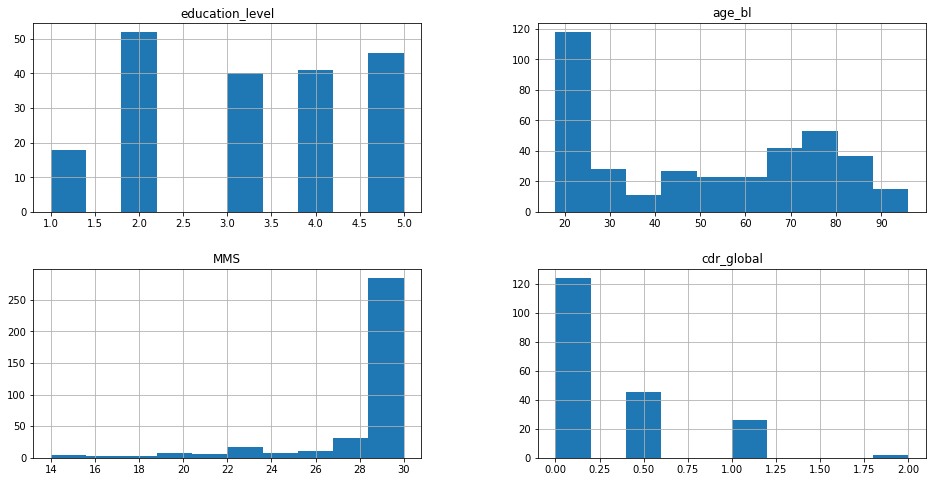
From these graphics, it’s possible to have an overview of the distribution of the data, for the numerical values. For example, the educational level is well distributed among the participants of the study. Also, most of the subjects are young (around 20 years old) and healthy (MMS score equals 30 and null CDR score).
The next cell will create (and run) a function (characteristics_table) that
highlights the main features of the population in the dataset. We will use it
later.
# Study the characteristics of the AD & CN populations (age, sex, MMS, cdr_global)
def characteristics_table(df, merged_df):
    """Creates a DataFrame that summarizes the characteristics of the DataFrame df"""
    diagnoses = np.unique(df.diagnosis.values)
    population_df = pd.DataFrame(index=diagnoses,
                                columns=['N', 'age', '%sexF', 'education',
                                         'MMS', 'CDR=0', 'CDR=0.5', 'CDR=1', 'CDR=2'])
    merged_df = merged_df.set_index(['participant_id', 'session_id'], drop=True)
    df = df.set_index(['participant_id', 'session_id'], drop=True)
    sub_merged_df = merged_df.loc[df.index]

    for diagnosis in population_df.index.values:
        diagnosis_df = sub_merged_df[df.diagnosis == diagnosis]
        population_df.loc[diagnosis, 'N'] = len(diagnosis_df)
        # Age
        mean_age = np.mean(diagnosis_df.age_bl)
        std_age = np.std(diagnosis_df.age_bl)
        population_df.loc[diagnosis, 'age'] = '%.1f ± %.1f' % (mean_age, std_age)
        # Sex
        population_df.loc[diagnosis, '%sexF'] = round((len(diagnosis_df[diagnosis_df.sex == 'F']) / len(diagnosis_df)) * 100, 1)
        # Education level
        mean_education_level = np.nanmean(diagnosis_df.education_level)
        std_education_level = np.nanstd(diagnosis_df.education_level)
        population_df.loc[diagnosis, 'education'] = '%.1f ± %.1f' % (mean_education_level, std_education_level)
        # MMS
        mean_MMS = np.mean(diagnosis_df.MMS)
        std_MMS = np.std(diagnosis_df.MMS)
        population_df.loc[diagnosis, 'MMS'] = '%.1f ± %.1f' % (mean_MMS, std_MMS)
        # CDR
        for value in ['0', '0.5', '1', '2']:
          population_df.loc[diagnosis, 'CDR=%s' % value] = len(diagnosis_df[diagnosis_df.cdr_global == float(value)])

    return population_df

population_df = characteristics_table(OASIS_df, OASIS_df)
population_df
| N | age | %sexF | education | MMS | CDR=0 | CDR=0.5 | CDR=1 | CDR=2 | |
|---|---|---|---|---|---|---|---|---|---|
| AD | 73 | 77.5 ± 7.4 | 63.0 | 2.7 ± 1.3 | 22.7 ± 3.6 | 0 | 45 | 26 | 2 |
| CN | 304 | 44.0 ± 23.3 | 62.2 | 3.5 ± 1.2 | 29.7 ± 0.6 | 124 | 0 | 0 | 0 |
Preprocessing
Theoretically, the main advantage of deep learning methods is to be able to work without extensive data preprocessing. However, as we have only a few images to train the network in this lab session, the preprocessing here is very extensive. More specifically, the images encountered:
Non-linear registration.
Segmentation of grey matter.
Conversion to tensor format (.pt).
As mentioned above, to obtain the preprocessed images, we used some pipelines provided by Clinica and ClinicaDL in order to:
Convert the original dataset to BIDS format (
clinica convert oasis-2-bids).Get the non-linear registration and segmentation of grey mater (pipeline
t1-volume).Obtain the preprocessed images in tensor format (tensor extraction using ClinicaDL,
clinicadl extract).
The preprocessed images are store in the CAPS
folder structure and all have
the same size (121x145x121). You will find below a class called MRIDataset
which allows easy browsing in the database.
from torch.utils.data import Dataset, DataLoader, sampler
from os import path

class MRIDataset(Dataset):

    def __init__(self, img_dir, data_df, transform=None):
        """
        Args:
            img_dir (str): path to the CAPS directory containing preprocessed images
            data_df (DataFrame): metadata of the population.
                Columns include participant_id, session_id and diagnosis).
            transform (callable): list of transforms applied on-the-fly, chained with torchvision.transforms.Compose.
        """
        self.img_dir = img_dir
        self.transform = transform
        self.data_df = data_df
        self.label_code = {"AD": 1, "CN": 0}

        self.size = self[0]['image'].shape

    def __len__(self):
        return len(self.data_df)

    def __getitem__(self, idx):

        diagnosis = self.data_df.loc[idx, 'diagnosis']
        label = self.label_code[diagnosis]

        participant_id = self.data_df.loc[idx, 'participant_id']
        session_id = self.data_df.loc[idx, 'session_id']
        filename = 'subjects/' + participant_id + '/' + session_id + '/' + \
          'deeplearning_prepare_data/image_based/custom/' + \
          participant_id + '_' + session_id + \
          '_T1w_segm-graymatter_space-Ixi549Space_modulated-off_probability.pt'

        image = torch.load(path.join(self.img_dir, filename))

        if self.transform:
            image = self.transform(image)

        sample = {'image': image, 'label': label,
                  'participant_id': participant_id,
                  'session_id': session_id}
        return sample

    def train(self):
        self.transform.train()

    def eval(self):
        self.transform.eval()
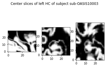
To facilitate the training and avoid overfitting due to the limited amount of data, the network won’t use the full image but only a part of the image (size 30x40x30) centered on a specific neuroanatomical region: the hippocampus (HC). This structure is known to be linked to memory, and is atrophied in the majority of cases of Alzheimer’s disease patients.
To improve the training and reduce overfitting, a random shift was added to the cropping function. This means that the bounding box around the hippocampus may be shifted by a limited amount of voxels in each of the three directions.
class CropLeftHC(object):
    """Crops the left hippocampus of a MRI non-linearly registered to MNI"""
    def __init__(self, random_shift=0):
        self.random_shift = random_shift
        self.train_mode = True
    def __call__(self, img):
        if self.train_mode:
            x = random.randint(-self.random_shift, self.random_shift)
            y = random.randint(-self.random_shift, self.random_shift)
            z = random.randint(-self.random_shift, self.random_shift)
        else:
            x, y, z = 0, 0, 0
        return img[:, 25 + x:55 + x,
                   50 + y:90 + y,
                   27 + z:57 + z].clone()

    def train(self):
        self.train_mode = True

    def eval(self):
        self.train_mode = False

class CropRightHC(object):
    """Crops the right hippocampus of a MRI non-linearly registered to MNI"""
    def __init__(self, random_shift=0):
        self.random_shift = random_shift
        self.train_mode = True
    def __call__(self, img):
        if self.train_mode:
            x = random.randint(-self.random_shift, self.random_shift)
            y = random.randint(-self.random_shift, self.random_shift)
            z = random.randint(-self.random_shift, self.random_shift)
        else:
            x, y, z = 0, 0, 0
        return img[:, 65 + x:95 + x,
                   50 + y:90 + y,
                   27 + z:57 + z].clone()

    def train(self):
        self.train_mode = True

    def eval(self):
        self.train_mode = False
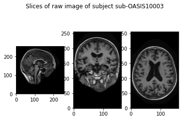
Visualization
Here we visualize the raw, preprocessed and cropped data.
import matplotlib.pyplot as plt
import nibabel as nib
from scipy.ndimage import rotate

subject = 'sub-OASIS10003'
preprocessed_pt = torch.load(f'OASIS-1_dataset/CAPS/subjects/{subject}/ses-M00/' +
                    f'deeplearning_prepare_data/image_based/custom/{subject}_ses-M00_' +
                    'T1w_segm-graymatter_space-Ixi549Space_modulated-off_' +
                    'probability.pt')
raw_nii = nib.load(f'OASIS-1_dataset/raw/{subject}_ses-M00_T1w.nii.gz')

raw_np = raw_nii.get_fdata()

def show_slices(slices):
    """ Function to display a row of image slices """
    fig, axes = plt.subplots(1, len(slices))
    for i, slice in enumerate(slices):
        axes[i].imshow(slice.T, cmap="gray", origin="lower")

slice_0 = raw_np[:, :, 78]
slice_1 = raw_np[122, :, :]
slice_2 = raw_np[:, 173, :]
show_slices([slice_0, rotate(slice_1, 90), rotate(slice_2, 90)])
plt.suptitle(f'Slices of raw image of subject {subject}')
plt.show()

slice_0 = preprocessed_pt[0, 60, :, :]
slice_1 = preprocessed_pt[0, :, 72, :]
slice_2 = preprocessed_pt[0, :, :, 60]
show_slices([slice_0, slice_1, slice_2])
plt.suptitle(f'Center slices of preprocessed image of subject {subject}')
plt.show()

leftHC_pt = CropLeftHC()(preprocessed_pt)
slice_0 = leftHC_pt[0, 15, :, :]
slice_1 = leftHC_pt[0, :, 20, :]
slice_2 = leftHC_pt[0, :, :, 15]
show_slices([slice_0, slice_1, slice_2])
plt.suptitle(f'Center slices of left HC of subject {subject}')
plt.show()

1. Cross-validation
In order to choose hyperparameters the set of images is divided into a training set (80%) and a validation set (20%). The data split was performed in order to ensure a similar distribution of diagnosis, age and sex between the subjects of the training set and the subjects of the validation set. Moreover the MMS distribution of each class is preserved.
train_df = pd.read_csv('OASIS-1_dataset/tsv_files/lab_1/train.tsv', sep='\t')
valid_df = pd.read_csv('OASIS-1_dataset/tsv_files/lab_1/validation.tsv', sep='\t')

train_population_df = characteristics_table(train_df, OASIS_df)
valid_population_df = characteristics_table(valid_df, OASIS_df)

print(f"Train dataset:\n {train_population_df}\n")
print(f"Validation dataset:\n {valid_population_df}")
Train dataset:
       N          age %sexF  education         MMS CDR=0 CDR=0.5 CDR=1 CDR=2
AD   58   77.4 ± 7.5  69.0  2.8 ± 1.4  22.6 ± 3.6     0      37    19     2
CN  242  43.4 ± 23.5  62.0  3.6 ± 1.2  29.8 ± 0.5    97       0     0     0

Validation dataset:
      N          age %sexF  education         MMS CDR=0 CDR=0.5 CDR=1 CDR=2
AD  15   78.2 ± 6.6  40.0  2.5 ± 1.0  22.9 ± 3.6     0       8     7     0
CN  62  46.3 ± 22.6  62.9  3.4 ± 1.3  29.6 ± 0.7    27       0     0     0
2. Model
We propose here to design a convolutional neural network that takes for input a patch centered on the left hippocampus of size 30x40x30. The architecture of the network was found using a Random Search on architecture + optimization hyperparameters.
Reminder on CNN layers
In a CNN everything is called a layer though the operations layers perform are very different. You will find below a summary of the different operations that may be performed in a CNN.
Feature maps
The outputs of the layers in a convolutional network are called feature maps. Their size is written with the format:
n_channels @ dim1 x dim2 x dim3
For a 3D CNN the dimension of the feature maps is actually 5D as the first
dimension is the batch size. This dimension is added by the DataLoader of
Pytorch which stacks the 4D tensors computed by a Dataset.
img_dir = path.join('OASIS-1_dataset', 'CAPS')
batch_size=4

example_dataset = MRIDataset(img_dir, OASIS_df, transform=CropLeftHC())
example_dataloader = DataLoader(example_dataset, batch_size=batch_size, drop_last=True)
for data in example_dataloader:
    pass

print(f"Shape of Dataset output:\n {example_dataset[0]['image'].shape}\n")

print(f"Shape of DataLoader output:\n {data['image'].shape}")
Shape of Dataset output:
 torch.Size([1, 30, 40, 30])

Shape of DataLoader output:
 torch.Size([4, 1, 30, 40, 30])
Convolutions (nn.Conv3d)
The main arguments of this layer are the input channels, the output channels
(number of filters trained) and the size of the filter (or kernel). If an
integer k is given the kernel will be a cube of size k. It is possible to
construct rectangular kernels by entering a tuple (but this is very rare).
You will find below an illustration of how a single filter produces its output feature map by parsing the one feature map. The size of the output feature map produced depends of the convolution parameters and can be computed with the following formula:
\(O_i = \frac{I_i-k+2P}{S} + 1\)
\(O_i\) the size of the output along the ith dimension
\(I_i\) the size of the input along the ith dimension
\(k\) the size of the kernel
\(P\) the padding value
\(S\) the stride value
In the following example \(\frac{5-3+2*0}{1}+1 = 3\)
To be able to parse all the feature maps of the input, one filter is actually
a 4D tensor of size (input_channels, k, k, k). The ensemble of all the
filters included in one convolutional layer is then a 5D tensor stacking all
the filters of size (output_channels, input_channels, k, k, k).
Each filter is also associated to one bias value that is a scalar added to
all the feature maps it produces. Then the bias is a 1D vector of size
output_channels.
from torch import nn

conv_layer = nn.Conv3d(8, 16, 3)
print('Weights shape\n', conv_layer.weight.shape)
print()
print('Bias shape\n', conv_layer.bias.shape)
Weights shape
 torch.Size([16, 8, 3, 3, 3])

Bias shape
 torch.Size([16])
Batch Normalization (nn.BatchNorm3d)
Learns to normalize feature maps according to (Ioffe & Szegedy, 2015). The following formula is applied on each feature map \(FM_i\):
\(FM^{normalized}_i = \frac{FM_i - mean(FM_i)}{\sqrt{var(FM_i) + \epsilon}} * \gamma_i + \beta_i\)
\(\epsilon\) is a hyperparameter of the layer (default=1e-05)
\(\gamma_i\) is the value of the scale for the ith channel (learnable parameter)
\(\beta_i\) is the value of the shift for the ith channel (learnable parameter)
This layer does not have the same behaviour during training and evaluation,
this is why it is needed to put the model in evaluation mode in the test
function with the command .eval()
batch_layer = nn.BatchNorm3d(16)
print('Gamma value\n', batch_layer.state_dict()['weight'].shape)
print()
print('Beta value\n', batch_layer.state_dict()['bias'].shape)
Gamma value
 torch.Size([16])

Beta value
 torch.Size([16])
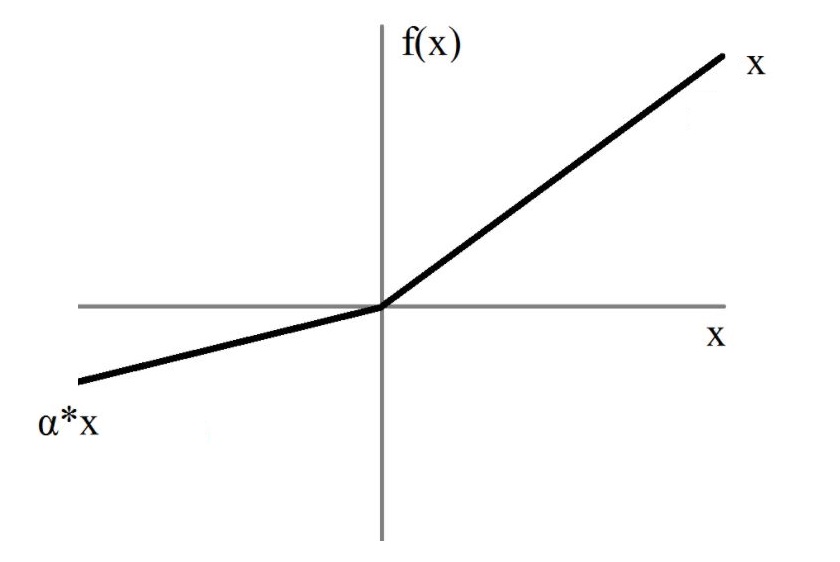
Activation function (nn.LeakyReLU)
In order to introduce non-linearity in the model, an activation function is introduced after the convolutions. It is applied on all intensities independently.
The graph of the Leaky ReLU is displayed below, \(\alpha\) being a hyperparameter of the layer (default=0.01):
Pooling function (PadMaxPool3d)
The structure of the pooling layer is very similar to the convolutional layer: a kernel is passing through the input with a defined size and stride. However there is no learnable parameters in this layer, the kernel outputing the maximum value of the part of the feature map it covers.
Here is an example in 2D of the standard layer of pytorch nn.MaxPool2d:
We can observe that the last column may not be used depending on the size of the kernel/input and stride value.
This is why the custom module PadMaxPool was defined to pad the input in
order to exploit information from the whole feature map.
class PadMaxPool3d(nn.Module):
    """A MaxPooling module which deals with odd sizes with padding"""
    def __init__(self, kernel_size, stride, return_indices=False, return_pad=False):
        super(PadMaxPool3d, self).__init__()
        self.kernel_size = kernel_size
        self.stride = stride
        self.pool = nn.MaxPool3d(kernel_size, stride, return_indices=return_indices)
        self.pad = nn.ConstantPad3d(padding=0, value=0)
        self.return_indices = return_indices
        self.return_pad = return_pad

    def set_new_return(self, return_indices=True, return_pad=True):
        self.return_indices = return_indices
        self.return_pad = return_pad
        self.pool.return_indices = return_indices

    def forward(self, f_maps):
        coords = [self.stride - f_maps.size(i + 2) % self.stride for i in range(3)]
        for i, coord in enumerate(coords):
            if coord == self.stride:
                coords[i] = 0

        self.pad.padding = (coords[2], 0, coords[1], 0, coords[0], 0)

        if self.return_indices:
            output, indices = self.pool(self.pad(f_maps))

            if self.return_pad:
                return output, indices, (coords[2], 0, coords[1], 0, coords[0], 0)
            else:
                return output, indices

        else:
            output = self.pool(self.pad(f_maps))

            if self.return_pad:
                return output, (coords[2], 0, coords[1], 0, coords[0], 0)
            else:
                return output
Here is an illustration of PadMaxPool behaviour. If the number of columns is odd, a column is added to avoid
losing data:
Similarly, the formula to find the size of the output feature map is:
\(O_i = ceil(\frac{I_i-k+2P}{S}) + 1\)
Dropout (nn.Dropout)
The aim of a dropout layer is to replace a fixed proportion of the input values by 0 during training only.
This layer does not have the same behaviour during training and evaluation,
this is why it is needed to put the model in evaluation mode in the test
function with the command .eval()
dropout = nn.Dropout(0.5)
input_tensor = torch.rand(10)
output_tensor = dropout(input_tensor)
print("Input \n", input_tensor)
print()
print("Output \n", output_tensor)
Input
 tensor([0.1311, 0.5546, 0.1405, 0.8767, 0.7725, 0.7001, 0.5156, 0.0886, 0.7068,
        0.1302])

Output
 tensor([0.0000, 1.1091, 0.2810, 0.0000, 1.5450, 0.0000, 1.0311, 0.1773, 1.4136,
        0.0000])
Fully-Connected Layers (nn.Linear)
The fully connected layers take as input 2D vectors of size (batch_size, N). They have two mandatory arguments, the number of values per batch of the
input and the number of values per batch of the output.
Each output neuron in a FC layer is a linear combination of the inputs + a bias.
fc = nn.Linear(16, 2)
print("Weights shape \n", fc.weight.shape)
print()
print("Bias shape \n", fc.bias.shape)
Weights shape
 torch.Size([2, 16])

Bias shape
 torch.Size([2])
TODO Network design
Construct here the network corresponding to the scheme and the following description:
The network includes 3 convolutional blocks composed by a convolutional layer (kernel size = 3, padding = 1, stride = 1), a batch normalization, a LeakyReLU activation and a MaxPooling layer. The 3 successive layers include respectively 8, 16 and 32 filters.
Then, the feature maps array is flattened in a 1D array to enter a fully-connected layer. Between the convolutional and the fully-connected layers, a dropout layer with a dropout rate of 0.5 is inserted.
# To complete
class CustomNetwork(nn.Module):

    def __init__(self):
        super(CustomNetwork, self).__init__()
        self.convolutions = nn.Sequential(
            nn.Conv3d(1, 8, 3, padding=1),
            # Size 8@30x40x30
            nn.BatchNorm3d(8),
            nn.LeakyReLU(),
            PadMaxPool3d(2, 2),
            # Size 8@15x20x15

            nn.Conv3d(8, 16, 3, padding=1),
            # Size 16@15x20x15
            nn.BatchNorm3d(16),
            nn.LeakyReLU(),
            PadMaxPool3d(2, 2),
            # Size 16@8x10x8)

            nn.Conv3d(16, 32, 3, padding=1),
            # Size 32@8x10x8
            nn.BatchNorm3d(32),
            nn.LeakyReLU(),
            PadMaxPool3d(2, 2),
            # Size 32@4x5x4

        )

        self.linear = nn.Sequential(
            nn.Dropout(p=0.5),
            nn.Linear(32 * 4 * 5 * 4, 2)

        )

    def forward(self, x):
        x = self.convolutions(x)
        x = x.view(x.size(0), -1)
        x = self.linear(x)
        return x
3. Train & Test
Complete the train method in order to iteratively update the weights of the
network.
Here the model leading to the lowest loss on the training set at the end of an epoch is returned, however we could choose instead the model leading to the highest balanced accuracy, or the one obtained at the last iteration.
In many studies of deep learning the validation set is used during training to choose when the training should stop (early stopping) but also to retrieve the best model (model selection).
As we don’t have any test set to evaluate the final model selected in an unbiased way, we chose not to use the validation set in training in order to limit the bias of the validation set. However you can choose to implement an early stopping and / or model selection based on the validation set, but remember that even if your results on the validation set are better, that doesn’t mean that this would be the case on an independent test set.
def train(model, train_loader, criterion, optimizer, n_epochs):
    """
    Method used to train a CNN

    Args:
        model: (nn.Module) the neural network
        train_loader: (DataLoader) a DataLoader wrapping a MRIDataset
        criterion: (nn.Module) a method to compute the loss of a mini-batch of images
        optimizer: (torch.optim) an optimization algorithm
        n_epochs: (int) number of epochs performed during training

    Returns:
        best_model: (nn.Module) the trained neural network
    """
    best_model = deepcopy(model)
    train_best_loss = np.inf

    for epoch in range(n_epochs):
        model.train()
        train_loader.dataset.train()
        for i, data in enumerate(train_loader, 0):
            # Retrieve mini-batch and put data on GPU with .cuda()
            images, labels = data['image'].cuda(), data['label'].cuda()
            # Forward pass
            outputs = model(images)
            # Loss computation
            loss = criterion(outputs, labels)
            # Back-propagation (gradients computation)
            loss.backward()
            # Parameters update
            optimizer.step()
            # Erase previous gradients
            optimizer.zero_grad()

        _, train_metrics = test(model, train_loader, criterion)

        print(
            f"Epoch {epoch}: loss = {train_metrics['mean_loss']:.4f}, "
            f"balanced accuracy = {train_metrics['balanced_accuracy']:.4f}"
            )

        if train_metrics['mean_loss'] < train_best_loss:
            best_model = deepcopy(model)
            train_best_loss = train_metrics['mean_loss']

    return best_model

def test(model, data_loader, criterion):
    """
    Method used to test a CNN

    Args:
        model: (nn.Module) the neural network
        data_loader: (DataLoader) a DataLoader wrapping a MRIDataset
        criterion: (nn.Module) a method to compute the loss of a mini-batch of images

    Returns:
        results_df: (DataFrame) the label predicted for every subject
        results_metrics: (dict) a set of metrics
    """
    model.eval()
    data_loader.dataset.eval()
    columns = ["participant_id", "proba0", "proba1",
               "true_label", "predicted_label"]
    results_df = pd.DataFrame(columns=columns)
    total_loss = 0

    with torch.no_grad():
        for i, data in enumerate(data_loader, 0):
            images, labels = data['image'].cuda(), data['label'].cuda()
            outputs = model(images)
            loss = criterion(outputs, labels)
            total_loss += loss.item()
            probs = nn.Softmax(dim=1)(outputs)
            _, predicted = torch.max(outputs.data, 1)

            for idx, sub in enumerate(data['participant_id']):
                row = [sub,
                       probs[idx, 0].item(), probs[idx, 1].item(),
                       labels[idx].item(), predicted[idx].item()]
                row_df = pd.DataFrame([row], columns=columns)
                results_df = pd.concat([results_df, row_df])

    results_metrics = compute_metrics(results_df.true_label.values, results_df.predicted_label.values)
    results_df.reset_index(inplace=True, drop=True)
    results_metrics['mean_loss'] = total_loss / len(data_loader.dataset)

    return results_df, results_metrics


def compute_metrics(ground_truth, prediction):
    """Computes the accuracy, sensitivity, specificity and balanced accuracy"""
    tp = np.sum((prediction == 1) & (ground_truth == 1))
    tn = np.sum((prediction == 0) & (ground_truth == 0))
    fp = np.sum((prediction == 1) & (ground_truth == 0))
    fn = np.sum((prediction == 0) & (ground_truth == 1))

    metrics_dict = dict()
    metrics_dict['accuracy'] = (tp + tn) / (tp + tn + fp + fn)

    # Sensitivity
    if tp + fn != 0:
        metrics_dict['sensitivity'] = tp / (tp + fn)
    else:
        metrics_dict['sensitivity'] = 0.0

    # Specificity
    if fp + tn != 0:
        metrics_dict['specificity'] = tn / (fp + tn)
    else:
        metrics_dict['specificity'] = 0.0

    metrics_dict['balanced_accuracy'] = (metrics_dict['sensitivity'] + metrics_dict['specificity']) / 2

    return metrics_dict
Train Classification with Left HC
Here we will train a first network that will learn to perform the binary classification AD vs CN on a cropped image around the left hippocampus.
All hyperparameters may have an influence, but one of the most influent is the learning rate that can lead to a poor convergence if it is too high or low. Try different learning rate between \(10 ^{-5}\) and \(10 ^{-3}\) and observe the differences of loss variations during training.
To increase the training speed you can also increase the batch size. But be careful, if the batch size becomes a non-negligible amount of the training set it may have a negative impact on loss convergence (Keskar et al, 2016).
Construction of dataset objects:
img_dir = path.join('OASIS-1_dataset', 'CAPS')
transform = CropLeftHC(2)

train_datasetLeftHC = MRIDataset(img_dir, train_df, transform=transform)
valid_datasetLeftHC = MRIDataset(img_dir, valid_df, transform=transform)

# Try different learning rates
learning_rate = 10**-4
n_epochs = 30
batch_size = 4

# Put the network on GPU
modelLeftHC = CustomNetwork().cuda()
train_loaderLeftHC = DataLoader(train_datasetLeftHC, batch_size=batch_size, shuffle=True, num_workers=8, pin_memory=True)
# A high batch size improves test speed
valid_loaderLeftHC = DataLoader(valid_datasetLeftHC, batch_size=32, shuffle=False, num_workers=8, pin_memory=True)
criterion = nn.CrossEntropyLoss(reduction='sum')
optimizer = torch.optim.Adam(modelLeftHC.parameters(), learning_rate)

best_modelLeftHC = train(modelLeftHC, train_loaderLeftHC, criterion, optimizer, n_epochs)

valid_resultsLeftHC_df, valid_metricsLeftHC = test(best_modelLeftHC, valid_loaderLeftHC, criterion)
train_resultsLeftHC_df, train_metricsLeftHC = test(best_modelLeftHC, train_loaderLeftHC, criterion)
print(valid_metricsLeftHC)
print(train_metricsLeftHC)
Epoch 0: loss = 0.3441, balanced accuracy = 0.5259
Epoch 1: loss = 0.2748, balanced accuracy = 0.6966
Epoch 2: loss = 0.3429, balanced accuracy = 0.5410
Epoch 3: loss = 0.2412, balanced accuracy = 0.7228
Epoch 4: loss = 0.2342, balanced accuracy = 0.7490
Epoch 5: loss = 0.2253, balanced accuracy = 0.7900
Epoch 6: loss = 0.2225, balanced accuracy = 0.7642
Epoch 7: loss = 0.2727, balanced accuracy = 0.8887
Epoch 8: loss = 0.2144, balanced accuracy = 0.7728
Epoch 9: loss = 0.2088, balanced accuracy = 0.7880
Epoch 10: loss = 0.2322, balanced accuracy = 0.8818
Epoch 11: loss = 0.2088, balanced accuracy = 0.7814
Epoch 12: loss = 0.2208, balanced accuracy = 0.8814
Epoch 13: loss = 0.2137, balanced accuracy = 0.7724
Epoch 14: loss = 0.2268, balanced accuracy = 0.8794
Epoch 15: loss = 0.2042, balanced accuracy = 0.7790
Epoch 16: loss = 0.2111, balanced accuracy = 0.8942
Epoch 17: loss = 0.1904, balanced accuracy = 0.8118
Epoch 18: loss = 0.1884, balanced accuracy = 0.8159
Epoch 19: loss = 0.1905, balanced accuracy = 0.7942
Epoch 20: loss = 0.2029, balanced accuracy = 0.7614
Epoch 21: loss = 0.1819, balanced accuracy = 0.7942
Epoch 22: loss = 0.1795, balanced accuracy = 0.8159
Epoch 23: loss = 0.1930, balanced accuracy = 0.7807
Epoch 24: loss = 0.2110, balanced accuracy = 0.9159
Epoch 25: loss = 0.1759, balanced accuracy = 0.8331
Epoch 26: loss = 0.1744, balanced accuracy = 0.8697
Epoch 27: loss = 0.1858, balanced accuracy = 0.7893
Epoch 28: loss = 0.1685, balanced accuracy = 0.8307
Epoch 29: loss = 0.2021, balanced accuracy = 0.9352
{'accuracy': 0.8831168831168831, 'sensitivity': 0.6, 'specificity': 0.9516129032258065, 'balanced_accuracy': 0.7758064516129033, 'mean_loss': 0.30914231670367254}
{'accuracy': 0.9066666666666666, 'sensitivity': 0.7068965517241379, 'specificity': 0.9545454545454546, 'balanced_accuracy': 0.8307210031347962, 'mean_loss': 0.16847280997782946}
If you obtained about 0.85 or more of balanced accuracy, there may be something wrong… Are you absolutely sure that your dataset is unbiased?
If you didn’t remove the youngest subjects of OASIS, your dataset is biased as the AD and CN participants do not have the same age distribution. In practice people who come to the hospital for a diagnosis of Alzheimer’s disease all have about the same age (50 - 90). No one has Alzheimer’s disease at 20 ! Then you should check that the performance of the network is still good for the old population only.
Check the accuracy on old participants (age > 62 to match the minimum of AD age distribution)
valid_resultsLeftHC_df = valid_resultsLeftHC_df.merge(OASIS_df, how='left', on='participant_id', sort=False)
valid_resultsLeftHC_old_df = valid_resultsLeftHC_df[(valid_resultsLeftHC_df.age_bl >= 62)]
compute_metrics(valid_resultsLeftHC_old_df.true_label, valid_resultsLeftHC_old_df.predicted_label)
{'accuracy': 0.71875,
 'sensitivity': 0.6,
 'specificity': 0.8235294117647058,
 'balanced_accuracy': 0.7117647058823529}
If the accuracy on old participants is very different from the one you obtained before, this could mean that your network is inefficient on the target population (persons older than 60). You have to think again about your framework and eventually retrain your network…
Train Classification with Right HC
Another network can be trained on a cropped image around the right HC network. The same hyperparameters as before may be reused.
Construction of dataset objects
transform = CropRightHC(2)

train_datasetRightHC = MRIDataset(img_dir, train_df, transform=transform)
valid_datasetRightHC = MRIDataset(img_dir, valid_df, transform=transform)

learning_rate = 10**-4
n_epochs = 30
batch_size = 4

# Put the network on GPU
modelRightHC = CustomNetwork().cuda()
train_loaderRightHC = DataLoader(train_datasetRightHC, batch_size=batch_size, shuffle=True, num_workers=8, pin_memory=True)
valid_loaderRightHC = DataLoader(valid_datasetRightHC, batch_size=32, shuffle=False, num_workers=8, pin_memory=True)
criterion = nn.CrossEntropyLoss(reduction='sum')
optimizer = torch.optim.Adam(modelRightHC.parameters(), learning_rate)

best_modelRightHC = train(modelRightHC, train_loaderRightHC, criterion, optimizer, n_epochs)

valid_resultsRightHC_df, valid_metricsRightHC = test(best_modelRightHC, valid_loaderRightHC, criterion)
train_resultsRightHC_df, train_metricsRightHC = test(best_modelRightHC, train_loaderRightHC, criterion)
print(valid_metricsRightHC)
print(train_metricsRightHC)
Epoch 0: loss = 0.3113, balanced accuracy = 0.5517
Epoch 1: loss = 0.2573, balanced accuracy = 0.7683
Epoch 2: loss = 0.2494, balanced accuracy = 0.7228
Epoch 3: loss = 0.2357, balanced accuracy = 0.7424
Epoch 4: loss = 0.2302, balanced accuracy = 0.7531
Epoch 5: loss = 0.2250, balanced accuracy = 0.7662
Epoch 6: loss = 0.2557, balanced accuracy = 0.9032
Epoch 7: loss = 0.2136, balanced accuracy = 0.8097
Epoch 8: loss = 0.2138, balanced accuracy = 0.8356
Epoch 9: loss = 0.2458, balanced accuracy = 0.9032
Epoch 10: loss = 0.2129, balanced accuracy = 0.7662
Epoch 11: loss = 0.2698, balanced accuracy = 0.9080
Epoch 12: loss = 0.2073, balanced accuracy = 0.8700
Epoch 13: loss = 0.2030, balanced accuracy = 0.8031
Epoch 14: loss = 0.2302, balanced accuracy = 0.8946
Epoch 15: loss = 0.2261, balanced accuracy = 0.8946
Epoch 16: loss = 0.2265, balanced accuracy = 0.7528
Epoch 17: loss = 0.2078, balanced accuracy = 0.7680
Epoch 18: loss = 0.1867, balanced accuracy = 0.8352
Epoch 19: loss = 0.2024, balanced accuracy = 0.9135
Epoch 20: loss = 0.1891, balanced accuracy = 0.9111
Epoch 21: loss = 0.1808, balanced accuracy = 0.8373
Epoch 22: loss = 0.1827, balanced accuracy = 0.8873
Epoch 23: loss = 0.1852, balanced accuracy = 0.8983
Epoch 24: loss = 0.1799, balanced accuracy = 0.8221
Epoch 25: loss = 0.1748, balanced accuracy = 0.8287
Epoch 26: loss = 0.1837, balanced accuracy = 0.9221
Epoch 27: loss = 0.2252, balanced accuracy = 0.7569
Epoch 28: loss = 0.1756, balanced accuracy = 0.8483
Epoch 29: loss = 0.1927, balanced accuracy = 0.9114
{'accuracy': 0.9090909090909091, 'sensitivity': 0.6666666666666666, 'specificity': 0.967741935483871, 'balanced_accuracy': 0.8172043010752688, 'mean_loss': 0.2644238243629406}
{'accuracy': 0.9033333333333333, 'sensitivity': 0.7068965517241379, 'specificity': 0.9504132231404959, 'balanced_accuracy': 0.828654887432317, 'mean_loss': 0.17483099497389049}
Soft voting
To increase the accuracy of our system the results of the two networks can be combined. Here we can give both hippocampi the same weight.
def softvoting(leftHC_df, rightHC_df):
    df1 = leftHC_df.set_index('participant_id', drop=True)
    df2 = rightHC_df.set_index('participant_id', drop=True)
    results_df = pd.DataFrame(index=df1.index.values,
                              columns=['true_label', 'predicted_label',
                                       'proba0', 'proba1'])
    results_df.true_label = df1.true_label
    # Compute predicted label and probabilities
    results_df.proba1 = 0.5 * df1.proba1 + 0.5 * df2.proba1
    results_df.proba0 = 0.5 * df1.proba0 + 0.5 * df2.proba0
    results_df.predicted_label = (0.5 * df1.proba1 + 0.5 * df2.proba1 > 0.5).astype(int)

    return results_df

valid_results = softvoting(valid_resultsLeftHC_df, valid_resultsRightHC_df)
valid_metrics = compute_metrics(valid_results.true_label, valid_results.predicted_label)
print(valid_metrics)
{'accuracy': 0.8961038961038961, 'sensitivity': 0.6666666666666666, 'specificity': 0.9516129032258065, 'balanced_accuracy': 0.8091397849462365}
Keep in mind that the validation set was used to set the hyperparameters (learning rate, architecture), then validation metrics are biased. To have unbiased results the entire framework should be evaluated on an independent set (test set).
4. Clustering on AD & CN populations
The classification results above were obtained in a supervised way: neurologists examine the participants of OASIS and gave a diagnosis depending on their clinical symptoms.
However, this label is often inaccurate (Beach et al, 2012). Then an unsupervised framework can be interesting to check what can be found in data without being biased by a noisy label.
Model
A convenient architecture to extract features from an image with deep learning is the autoencoder (AE). This architecture is made of two parts:
the encoder which learns to compress the image in a smaller vector, the code. It is composed of the same kind of operations than the convolutional part of the CNN seen before.
the decoder which learns to reconstruct the original image from the code learnt by the encoder. It is composed of the transposed version of the operations used in the encoder.
You will find below CropMaxUnpool3d the transposed version of
PadMaxPool3d.
class CropMaxUnpool3d(nn.Module):
    def __init__(self, kernel_size, stride):
        super(CropMaxUnpool3d, self).__init__()
        self.unpool = nn.MaxUnpool3d(kernel_size, stride)

    def forward(self, f_maps, indices, padding=None):
        output = self.unpool(f_maps, indices)
        if padding is not None:
            x1 = padding[4]
            y1 = padding[2]
            z1 = padding[0]
            output = output[:, :, x1::, y1::, z1::]

        return output
To facilitate the reconstruction process, the pooling layers in the encoder return the position of the values that were the maximum. Hence the unpooling layer can replace the maximum values at the right place in the 2x2x2 sub-cube of the feature map. They also indicate if some zero padding was applied to the feature map so that the unpooling layer can correctly crop their output feature map.
class AutoEncoder(nn.Module):

    def __init__(self):
        super(AutoEncoder, self).__init__()

        # Initial size (30, 40, 30)

        self.encoder = nn.Sequential(
            nn.Conv3d(1, 8, 3, padding=1),
            nn.BatchNorm3d(8),
            nn.LeakyReLU(),
            PadMaxPool3d(2, 2, return_indices=True, return_pad=True),
            # Size (15, 20, 15)

            nn.Conv3d(8, 16, 3, padding=1),
            nn.BatchNorm3d(16),
            nn.LeakyReLU(),
            PadMaxPool3d(2, 2, return_indices=True, return_pad=True),
            # Size (8, 10, 8)

            nn.Conv3d(16, 32, 3, padding=1),
            nn.BatchNorm3d(32),
            nn.LeakyReLU(),
            PadMaxPool3d(2, 2, return_indices=True, return_pad=True),
            # Size (4, 5, 4)

            nn.Conv3d(32, 1, 1),
            # Size (4, 5, 4)
        )

        self.decoder = nn.Sequential(
            nn.ConvTranspose3d(1, 32, 1),
            # Size (4, 5, 4)

            CropMaxUnpool3d(2, 2),
            nn.ConvTranspose3d(32, 16, 3, padding=1),
            nn.BatchNorm3d(16),
            nn.LeakyReLU(),
            # Size (8, 10, 8)

            CropMaxUnpool3d(2, 2),
            nn.ConvTranspose3d(16, 8, 3, padding=1),
            nn.BatchNorm3d(8),
            nn.LeakyReLU(),
            # Size (15, 20, 15)

            CropMaxUnpool3d(2, 2),
            nn.ConvTranspose3d(8, 1, 3, padding=1),
            nn.BatchNorm3d(1),
            nn.Sigmoid()
            # Size (30, 40, 30)
        )

    def forward(self, x):
        indices_list = []
        pad_list = []
        for layer in self.encoder:
            if isinstance(layer, PadMaxPool3d):
                x, indices, pad = layer(x)
                indices_list.append(indices)
                pad_list.append(pad)
            else:
                x = layer(x)

        code = x.view(x.size(0), -1)
        for layer in self.decoder:
            if isinstance(layer, CropMaxUnpool3d):
                x = layer(x, indices_list.pop(), pad_list.pop())
            else:
                x = layer(x)

        return code, x
Train Autoencoder
The training function of the autoencoder is very similar to the training function of the CNN. The main difference is that the loss is not computed by comparing the output with the diagnosis values using the cross-entropy loss, but with the original image using for example the Mean Squared Error (MSE) loss.
def trainAE(model, train_loader, criterion, optimizer, n_epochs):
    """
    Method used to train an AutoEncoder

    Args:
        model: (nn.Module) the neural network
        train_loader: (DataLoader) a DataLoader wrapping a MRIDataset
        criterion: (nn.Module) a method to compute the loss of a mini-batch of images
        optimizer: (torch.optim) an optimization algorithm
        n_epochs: (int) number of epochs performed during training

    Returns:
        best_model: (nn.Module) the trained neural network.
    """
    best_model = deepcopy(model)
    train_best_loss = np.inf

    for epoch in range(n_epochs):
        model.train()
        train_loader.dataset.train()
        for i, data in enumerate(train_loader, 0):
            # ToDo
            # Complete the training function in a similar way
            # than for the CNN classification training.
            # Retrieve mini-batch
            images, labels = data['image'].cuda(), data['label'].cuda()
            # Forward pass + loss computation
            _, outputs = model((images))
            loss = criterion(outputs, images)
            # Back-propagation
            loss.backward()
            # Parameters update
            optimizer.step()
            # Erase previous gradients
            optimizer.zero_grad()

        mean_loss = testAE(model, train_loader, criterion)

        print(f'Epoch {epoch}: loss = {mean_loss:.6f}')

        if mean_loss < train_best_loss:
            best_model = deepcopy(model)
            train_best_loss = mean_loss

    return best_model


def testAE(model, data_loader, criterion):
    """
    Method used to test an AutoEncoder

    Args:
        model: (nn.Module) the neural network
        data_loader: (DataLoader) a DataLoader wrapping a MRIDataset
        criterion: (nn.Module) a method to compute the loss of a mini-batch of images

    Returns:
        results_df: (DataFrame) the label predicted for every subject
        results_metrics: (dict) a set of metrics
    """
    model.eval()
    data_loader.dataset.eval()
    total_loss = 0

    with torch.no_grad():
        for i, data in enumerate(data_loader, 0):
            images, labels = data['image'].cuda(), data['label'].cuda()
            _, outputs = model((images))
            loss = criterion(outputs, images)
            total_loss += loss.item()

    return total_loss / len(data_loader.dataset) / np.product(data_loader.dataset.size)
learning_rate = 10**-3
n_epochs = 30
batch_size = 4

AELeftHC = AutoEncoder().cuda()
criterion = nn.MSELoss(reduction='sum')
optimizer = torch.optim.Adam(AELeftHC.parameters(), learning_rate)

best_AELeftHC = trainAE(AELeftHC, train_loaderLeftHC, criterion, optimizer, n_epochs)
Epoch 0: loss = 0.092463
Epoch 1: loss = 0.057393
Epoch 2: loss = 0.046466
Epoch 3: loss = 0.039317
Epoch 4: loss = 0.035276
Epoch 5: loss = 0.031526
Epoch 6: loss = 0.028902
Epoch 7: loss = 0.026990
Epoch 8: loss = 0.025812
Epoch 9: loss = 0.023425
Epoch 10: loss = 0.022873
Epoch 11: loss = 0.020765
Epoch 12: loss = 0.019893
Epoch 13: loss = 0.019150
Epoch 14: loss = 0.018286
Epoch 15: loss = 0.017654
Epoch 16: loss = 0.017210
Epoch 17: loss = 0.017415
Epoch 18: loss = 0.016208
Epoch 19: loss = 0.015972
Epoch 20: loss = 0.015389
Epoch 21: loss = 0.015128
Epoch 22: loss = 0.014811
Epoch 23: loss = 0.014832
Epoch 24: loss = 0.014468
Epoch 25: loss = 0.014108
Epoch 26: loss = 0.014059
Epoch 27: loss = 0.013753
Epoch 28: loss = 0.013487
Epoch 29: loss = 0.013449
Visualization
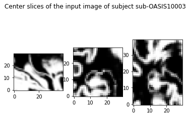
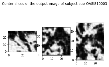
The simplest way to check if the AE training went well is to visualize the output and compare it to the original image seen by the autoencoder.
import matplotlib.pyplot as plt
import nibabel as nib
from scipy.ndimage import rotate

subject = 'sub-OASIS10003'
preprocessed_pt = torch.load(f'OASIS-1_dataset/CAPS/subjects/{subject}/ses-M00/' +
                    'deeplearning_prepare_data/image_based/custom/' + subject +
                    '_ses-M00_'+
                    'T1w_segm-graymatter_space-Ixi549Space_modulated-off_' +
                    'probability.pt')
input_pt = CropLeftHC()(preprocessed_pt).unsqueeze(0).cuda()
_, output_pt = best_AELeftHC(input_pt)


slice_0 = input_pt[0, 0, 15, :, :].cpu()
slice_1 = input_pt[0, 0, :, 20, :].cpu()
slice_2 = input_pt[0, 0, :, :, 15].cpu()
show_slices([slice_0, slice_1, slice_2])
plt.suptitle(f'Center slices of the input image of subject {subject}')
plt.show()

slice_0 = output_pt[0, 0, 15, :, :].cpu().detach()
slice_1 = output_pt[0, 0, :, 20, :].cpu().detach()
slice_2 = output_pt[0, 0, :, :, 15].cpu().detach()
show_slices([slice_0, slice_1, slice_2])
plt.suptitle(f'Center slices of the output image of subject {subject}')
plt.show()
Clustering
Now that the AE extracted the most salient parts of the image in a smaller vector, the features obtained can be used for clustering.
Here we give an example with the Gaussian Mixture Model (GMM) of
scikit-learn. To use it we first need to concat the features and the labels
of all the subjects in two matrices X and Y. This is what is done in
compute_dataset_features method.
def compute_dataset_features(data_loader, model):

    concat_codes = torch.Tensor().cuda()
    concat_labels = torch.LongTensor()
    concat_names = []

    for data in data_loader:
      image = data['image'].cuda()
      labels = data['label']
      names = data['participant_id']

      code, _ = model(image)
      concat_codes = torch.cat([concat_codes, code.squeeze(1)], 0)
      concat_labels = torch.cat([concat_labels, labels])
      concat_names = concat_names + names

    concat_codes_np = concat_codes.cpu().detach().numpy()
    concat_labels_np = concat_labels.numpy()
    concat_names = np.array(concat_names)[:, np.newaxis]

    return concat_codes_np, concat_labels_np, concat_names
# train_codes, train_labels, names = compute_dataset_features(train_loaderBothHC, best_AEBothHC)
train_codes, train_labels, names = compute_dataset_features(train_loaderLeftHC, best_AELeftHC)
Then the model will fit the training codes and build two clusters. The labels found in this unsupervised way can be compared to the true labels.
from sklearn import mixture
from sklearn.metrics import adjusted_rand_score

n_components = 2
model = mixture.GaussianMixture(n_components)
model.fit(train_codes)
train_predict = model.predict(train_codes)

metrics = compute_metrics(train_labels, train_predict)
ari = adjusted_rand_score(train_labels, train_predict)
print(f"Adjusted random index: {ari}")
Adjusted random index: 0.33869103831169145
The adjusted random index may not be very good, this could mean that the framework clustered another characteristic that the one you tried to target.
What is actually expected is that the clustering differenciation is made on the level of atrophy, which is mostly correlated to the age but also to the disease stage (we can model it with the MMS score).
data_np = np.concatenate([names, train_codes,
                          train_labels[:, np.newaxis],
                          train_predict[:, np.newaxis]], axis=1)
columns = ['feature %i' % i for i in range(train_codes.shape[1])]
columns = ['participant_id'] + columns + ['true_label', 'predicted_label']
data_df = pd.DataFrame(data_np, columns=columns).set_index('participant_id')

merged_df = data_df.merge(OASIS_df.set_index('participant_id'), how='inner', on='participant_id')

plt.title('Clustering values according to age and MMS score')
for component in range(n_components):
    predict_df = merged_df[merged_df.predicted_label == str(component)]
    plt.plot(predict_df['age_bl'], predict_df['MMS'], 'o', label=f"cluster {component}")
plt.legend()
plt.xlabel('age')
plt.ylabel('MMS')
plt.show()
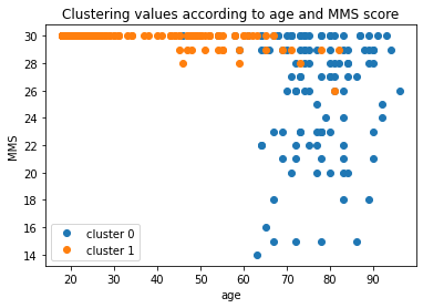
You can try to improve this clustering by adding the codes obtained on the right hippocampus, perform further dimension reduction or remove age effect like in (Moradi et al, 2015)…